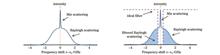
ObjectiveAmong the myriad factors influencing climate change, the interaction between clouds and aerosols is the most uncertain element in global climate dynamics, and is widely acknowledged as a formidable challenge in atmospheric science. High-spectral-resolution lidar (HSRL) observations of vertical distribution characteristics of clouds and aerosols, independent of assumptions about cloud vertical structure and lidar ratio, hold immense scientific potential for future research on cloud-aerosol interactions. In HSRL systems, active frequency locking technology is typically employed to match the emitted laser wavelength with the etalon, thus ensuring system parameter stability. However, changes in the working environment or hardware failures can reduce the locking precision to significantly degrade the high-spectral-resolution detection performance. Therefore, real-time calibration of molecular transmittance, correction of detection results, and enhancement of detection accuracy are of paramount significance.MethodsIn the HSRL system, the molecular transmittance is determined by the collaboration of multiple components such as the emitted laser and the etalon. Ground-based lidar observations are susceptible to environmental changes, which require timely calibration for accurate inversion. The atmosphere is replete with a multitude of components such as clouds and aerosols, necessitating stratified identification. Distinguishing between clouds, aerosols, and clean areas in the atmosphere lays the foundation for calibrating molecular transmittance. We introduce an online method for calibrating molecular transmittance, which avoids interference from clouds and aerosols by stratified identification to achieve online calibration of molecular transmittance. Since the proposed HSRL can directly invert atmospheric optical property parameters without assuming a lidar ratio, the utilization of a scattering ratio threshold method for classification provides unique advantages.Results and DiscussionsThe experiment selects calibration cases in three distinct atmospheric conditions in Beijing, including clear, dusty, and cloudy conditions. Under these different atmospheric states, molecular transmittance calibration can be performed by following atmospheric stratified identification, which demonstrates that this method can calibrate molecular transmittance in various weather conditions. To verify the accuracy of the HSRL detection results, we compare the HSRL with the widely employed sun photometer. The observation results in Beijing are inverted by adopting both fixed molecular transmittance and online calibration parameters. When fixed parameters are leveraged for inversion, the correlation coefficient of the detection results of the two instruments is 0.92, and the root mean square error is 0.136. After conducting correction with this method, some inversion errors are effectively corrected, the correlation coefficient reaches 0.94, and the root mean square error decreases to 0.078. The detection results obtained from the inversion show higher consistency with that of the sun photometer.ConclusionsWe initially analyze the molecular transmittance error based on the fundamental principles and detection methods of HSRL. In the HSRL system, where an iodine molecule absorption cell serves as a spectral etalon, the systematic error in molecular transmittance primarily results from the frequency fluctuation of the emitted laser and temperature instability in the molecular absorption cell. Meanwhile, an online calibration method for molecular transmittance is proposed to rectify the influence caused by system instability. Unlike the calibration method that fixes clean atmospheric areas, this method exploits the HSRL characteristics that can simply and accurately invert the backscatter ratio, and employs the backscatter ratio as the basis for stratified identification. Additionally, after selecting clean areas in the atmosphere, the molecular transmittance is calibrated by adopting these clean areas. This leads to the result that transmittance calibration cannot be limited to clear weather, thus supplementing the calibration method in non-clear weather conditions. Finally, based on the observation results of the HSRL system in Beijing, an analysis of its observation results is conducted to demonstrate the effectiveness of this method in enhancing detection accuracy.

ObjectiveClouds play a crucial role as intermediary factors in maintaining the balance of atmospheric radiation energy and water cycle. The particle size distribution (PSD) and the optical and microphysical properties of clouds are intricately linked. Therefore, precise determination of PSD is pivotal for analyzing the interactions among different atmospheric components. Polarized remote sensing, a novel atmospheric detection technology, can be utilized to retrieve the PSD of water clouds. Multi-directional observation information can be leveraged to retrieve PSD. However, current methods overlook sensor scattering angle coverage and actual cloud characteristics. The fixed-resolution sampling method within the field of view (FOV) neglects the influence of sensor imaging characteristics and cloud heterogeneity. Therefore, conducting studies aimed at enhancing the accuracy of water PSD inversion based on sensor imaging and cloud characteristics is important for atmospheric research.MethodsIn PSD retrieval research using polarized multi-angle observation data, the selection of inversion scale significantly influences the number of available observation angles and the cloud’s heterogeneity. To address these limitations, we propose a dynamic scale PSD retrieval method based on multi-angle polarized data, leveraging the polarized radiation characteristics of water clouds and radiation transmission theory. We conduct a quantitative evaluation of retrieval feasibility at various scales within satellite imaging geometry and cloud characteristics. Our method utilizes an optimal pixel merging strategy at a pixel-by-pixel level to improve inversion resolution while maintaining accuracy, ultimately applying the inversion method to directional polarization camera (DPC) observation data. Results indicate that, unlike the fixed retrieval scale of 25 pixel×25 pixel used in POLDER (polarization and directionality of the Earth’s reflectance) product, our method dynamically adjusts the inversion scale between 1 pixel×1 pixel and 7 pixel×7 pixel, leading to improved retrieval resolution. Thus, the optimization strategy for inversion scale in this study aims to strike the best balance between inversion success rate and accuracy, employing a dynamic selection method on a pixel-by-pixel basis. Tailored to the imaging characteristics of domestically produced DPC data, we devise the technical flowchart depicted in Fig. 1. Initially, we establish a polarized scattering phase function library for various water cloud droplet PSDs. By considering the number of observed angles within the water cloud “rainbow” effect among DPC observations, we determine the initial inversion scale. Simultaneously, we iteratively optimize the inversion resolution based on the number of observed angles and cloud attribute information within the scale. Finally, by leveraging multi-angle polarized observation data, we achieve the inversion of water cloud droplet size distributions at the optimal inversion scale.Results and DiscussionsCompared with moderate resolution imaging spectroradiometer (MODIS) cloud effective particle radius products, the spatial distribution shows good consistency. As depicted in Fig. 8, the inversion results of overlapping areas between MOD06~~L2.A2022068.0220.061.20220 and DPC are contrasted within the case study region. Figures 8(a) and 8(b) vividly depict that the values and distributions of cloud effective particle radius from DPC and MODIS exhibit remarkable similarity. However, Fig. 8(c) reveals substantial disparities in inversion values between the two, primarily in fragmented cloud regions, whereas variances in stable cloud cluster areas are negligible. In Fig. 9, we perform a quantitative statistical analysis of the inversion results within overlapping areas. Using regression equations derived from fitting, our inversion results yield smaller values for cloud effective particle radius compared to MODIS products, especially for radius of 5?12 μm. This trend aligns with comparisons between POLDER and MODIS. For larger particles, both DPC and inversion results surpass those of MODIS, possibly due to lower sensitivity of polarization to larger particles, leading to increased inversion errors for this particle size range. In histogram analysis, the proportion of inversion results with errors less than 2.05 μm exceeds 50%. Considering significant differences in imaging time between DPC and MODIS, substantial shifts in cloud position, variations in shape, and disparities in sensor resolution and inversion methods, significant errors in pixel-by-pixel comparisons are expected. However, these deviations are acceptable. Therefore, analyses indicate our method can yield more detailed inversion results while maintaining high accuracy.ConclusionsThe dynamic inversion resolution method improves upon conventional techniques by considering the variations in scattering angle coverage across different regions and the effect of cloud structures on satellite wide FOV imaging. By carefully considering observational conditions and the real-time state of clouds at a pixel level, this method avoids loss of accuracy and success rate stemming from arbitrary resolution selection in PSD inversion. Additionally, it reduces uncertainties from geometric variations in multi-angle imaging and cloud heterogeneity during inversion. Consequently, our study provides significant benefits in enhancing the accuracy and success rate of cloud PSD retrieval. In conclusion, our research explores ways to enhance the efficiency of utilizing domestic multi-angle polarized data and improve the accuracy of PSD inversion.

ObjectiveAs a new type of active remote sensing equipment, lidar is increasingly widely used in the measurement of atmospheric components such as aerosols, water vapor, and ozone. Raman lidar used for aerosol and water vapor detection has outstanding advantages such as high detection accuracy, high spatiotemporal resolution, and real-time measurement capabilities. It is suitable for various mobile platforms such as vehicle mounted and airborne systems and has become one of the main technical means for accurately detecting the distribution of atmospheric aerosols and water vapor. The receiving field of view of a lidar cannot completely coincide with the laser beam at close range. The laser beam gradually enters the receiving field of view, so the echo signal received by the lidar at close range is only a partial echo signal of the laser beam. To describe this effect, a geometric overlap factor, abbreviated as the geometric factor, is defined. Due to the influence of geometric factors, the measurement results of lidar in the close range geometric factor area are inaccurate. The closer the distance, the more significant this effect becomes. Since atmospheric water vapor is mainly distributed below the troposphere, if we want to use lidar to obtain accurate water vapor distribution profiles, it is necessary to calibrate and calculate the geometric factors. This article focuses on the situation where the receiving telescope’s field of view is partially obstructed by obstacles during horizontal experimental measurement of geometric factors in the practical application of gas-soluble glue water vapor Raman lidar. We have made some improvements to the correction method of geometric factors.MethodsWe propose an improved geometric factor correction method to solve the problem of partial occlusion of the telescope’s receiving field of view in horizontal experimental measurements of gas-soluble glue water vapor Raman lidar. This method is based on the experimental method commonly used for geometric factor correction, which involves measuring the lidar along the horizontal direction under horizontally uniform atmospheric conditions. Improvements have been made to the experimental scheme and data processing methods. Firstly, a shading device is used to completely block the lower half of the telescope’s field of view (Fig. 2). The position of the shading device can be flexibly adjusted according to the occlusion of the object, ensuring that the unobstructed part can be fully received on the path. The improved experimental plan is as follows: ① a shading device is used to cover half of the received field of view of the telescope, followed by horizontal measurement with a lidar in the azimuth direction under good visibility conditions; ② the pitch angle is adjusted to 90°, ensuring the shading device in an unobstructed state for a set of vertical measurements with the same parameters; ③ the shading device is quickly removed to perform another set of vertical measurements under the same conditions. To obtain the geometric factor of the lidar before the method improvement, distance squared correction is applied to the echo signal measured horizontally by the lidar in the first step. An appropriate linear range is then selected for fitting [Fig. 4(a)], and the ratio of the two measurements is processed to determine the geometric factor [Fig. 4(b)]. Since the occlusion state of the telescope remains unchanged during horizontal measurement in step ① and vertical measurement in step ②, the geometric factors processed in step ① can be used for correcting the vertical occlusion measurement echo signal in step ② (Fig. 5). In step ③, the shading device is quickly removed to perform a set of vertical measurements with the same parameters as in step ②. The interval between the two vertical measurements is very short, allowing the assumption that the atmospheric state remains unchanged. The echo signal of the vertical unobstructed measurement without geometric factor correction in step ③ and the echo signal of the vertical unobstructed measurement with geometric factor correction in step ② are plotted together (Fig. 6). Normalizing the ratio of the two signals provides the true and accurate geometric factor of the aerosol water vapor Raman lidar (Fig. 7).Results and DiscussionsContinuous atmospheric observation experiments are conducted using a self-developed aerosol water vapor Raman lidar system, and the extinction coefficient profiles of aerosols before and after geometric factor correction using the improved method are inverted (Fig. 10). We compare and analyze the calculation results of the 532 nm wavelength optical thickness of the lidar before and after the improvement of the geometric factor correction method with the continuous measurement results of the 550 nm wavelength optical thickness of the solar radiometer at the same time and space (Fig. 11). The correlation analysis results show that the correlation coefficient between the improved geometric factor correction method and the measurement results of the lidar and solar radiometer is as high as 0.9779 (Fig. 12), indicating good consistency between the two. From the calculation results of relative error, the relative error between the improved lidar optical thickness (532 nm) calculation results and the solar radiometer (550 nm) measurement results is within 10%, with an average relative error of 3.81% and a maximum relative error of 8.23%. The average relative error before the method improvement is 8.34%, and the maximum relative error is 18.26%. The accuracy of the improved method is 2.19 times that of the original method. The reliability of the lidar measurement results and the rationality and accuracy of the improved geometric factor correction method have been fully verified.ConclusionsWe calculate and analyze the correction effect of the proposed improved geometric factor correction method. The results indicate that this method can accurately calculate the geometric factors of Raman lidar systems under partial occlusion conditions. After the geometric factor correction obtained by the improved method, the accuracy and reliability of the lidar measurement results are good. The improved geometric factor correction method has a certain reference value for the practical application of aerosol water vapor Raman lidar systems.

ObjectiveHigh spatiotemporal resolution atmospheric wind field detection has important applications in pollution transport and diffusion, extreme weather monitoring, numerical weather forecasting, wind resource assessment, and other areas. Coherent Doppler lidar, as an active laser remote sensing device, acquires high spatiotemporal resolution vector wind field vertical-structure information. However, in practical applications, factors such as platform or power supply stability, and weather conditions can lead to missing wind profiles, limiting the application scope of wind-sensing lidar. Deep learning methods based on historical data modeling have been widely used in wind field prediction. The long short-term memory (LSTM) network shows good performance in wind field prediction. However, most studies mainly focus on one-dimensional temporal or spatial wind fields, while atmospheric wind fields exhibit both temporal and vertical spatial characteristics. Doppler lidar, as a high spatiotemporal resolution atmospheric wind field detection tool, obtains spatiotemporal two-dimensional wind field information. Therefore, we propose a method using a bidirectional long short-term memory (Bi-LSTM) model applied to wind field detection with lidar for wind profile prediction. The aim is to fully utilize the spatiotemporal two-dimensional wind field data observed by the lidar, train a temporal Bi-LSTM model to capture the temporal variation characteristics of wind profiles, predict future wind profiles, interpolate missing wind profiles, and acquire more continuous wind field information.MethodsOur study focuses on Doppler lidar atmospheric wind field detection experiments in Juehua Island, Liaoning Province, China. We utilize complete wind profile data for modeling and validation to predict and interpolate deficient wind profiles detected by the lidar. Previous complete wind profile data segments serve as the training and validation sets to establish wind profile prediction models based on a time-series Bi-LSTM model and a non-time series convolutional neural network (CNN) model for the zonal component u and meridional component v of the wind profiles. We train the models using the same parameter settings, including step size, number of iterations, loss function, and optimization algorithm. We evaluate the wind profile prediction performance of the Bi-LSTM and CNN models using various metrics such as coefficient of determination (R2), root mean square error (RMSE), and mean absolute error (MAE). The Bi-LSTM model with superior validation wind profile prediction performance is then used for deficient wind profile prediction and interpolation to obtain more continuous wind field information.Results and DiscussionsBased on the evaluation results of wind profile prediction (Fig. 4), the Bi-LSTM model shows similar trends and ranges in performance evaluation metrics R2, RMSE, and MAE for different look-back steps. As a temporal network, the Bi-LSTM model exhibits consistent performance across different look-back steps, indicating that wind profiles have short-term or long-term temporal dependencies that allow prediction based on past wind profiles at various time steps. With an increase in prediction time steps, errors accumulate gradually. After the 16th time step iteration, the model’s predictive capability rapidly declines, with R2 values for predicting u and v components falling below 0.5, indicating an inability to accurately forecast wind profiles beyond that point. This suggests that the Bi-LSTM model demonstrates good short-term predictive ability for the next 15 wind profiles (within the next 2.5 h). Comparing the wind profile prediction performance of the temporal Bi-LSTM model with the non-temporal CNN model, the box plot analysis (Fig. 5) reveals that the CNN model shows greater variability in R2 values for wind profile prediction across different look-backs, indicating a more pronounced influence of the look-back parameter on wind profile prediction and greater uncertainty introduced by the choice of look-backs. The Bi-LSTM model outperforms the CNN model in predicting u and v profiles, likely due to its ability to capture temporal features of wind profiles. In short-term wind prediction, the Bi-LSTM model exhibits lower variability in R2 values across different look-backs, demonstrating greater robustness in wind profile prediction. Compared to the CNN model, the Bi-LSTM model achieves higher R2 values and lower errors in prediction. The differences in predictive performance may stem from the CNN model’s proficiency in extracting local features using convolutional kernels, while wind profiles, as time series data, exhibit features closely related to preceding and subsequent time steps, potentially limiting the CNN model’s performance in handling such time-dependent wind profile data. In contrast, the Bi-LSTM network, with bidirectional LSTM layers, considers features of wind profiles from multiple time steps in both directions, enabling it to better capture dependencies in time series data and make more accurate wind profile predictions. Future work involves incorporating time-series data such as boundary layer height, temperature, humidity, and pressure as input features to further explore the Bi-LSTM model’s wind profile prediction performance (Fig. 8). Additionally, we find it necessary to increase the number of training time steps to achieve better wind profile prediction results.ConclusionsIn the present study, we propose a method for wind profile prediction using a Bi-LSTM model applied to wind field detection with lidar. The aim is to fully utilize the spatiotemporal two-dimensional wind field data observed by the lidar. By training a temporal Bi-LSTM model to extract the temporal variations of wind profiles, we predict future wind profiles and interpolate missing wind profiles. We conduct a comparison between the temporal Bi-LSTM model and the non-temporal CNN model in wind profile prediction. Our study reveals that the temporal Bi-LSTM model exhibits higher robustness in short-term wind field prediction compared to the non-temporal CNN model.

ObjectiveNitrogen dioxide (NO2) not only directly affects air quality and participates in secondary chemical reactions but also influences human health. It primarily originates from industrial and vehicular emissions, as well as regional transport at higher altitudes. Therefore, surface in situ measurements alone cannot fully comprehend the high-altitude transport, vertical evolution, and atmospheric chemical processes of NO2. In this study, we aim to investigate the vertical distribution characteristics and temporal variations of NO2 in Beijing, given its status as a primary atmospheric pollutant originating from industrial activities and vehicular emissions. With Beijing’s dense population and high vehicle density, vehicular emissions constitute a major source of NO2. Despite improvements in air quality due to environmental policies, regional transport, especially along the southwest?northeast corridor, remains a significant contributor to NO2 levels in Beijing. Traditional monitoring methods have limitations in capturing NO2 transport dynamics, necessitating advanced techniques such as multi-axis differential optical absorption spectroscopy (MAX-DOAS). This research, based on two years of MAX-DOAS observations, is designed to understand NO2’s vertical distribution and its response to policy interventions and holiday effects. By providing detailed insights into NO2 behavior under various conditions, we support effective air quality management and policy formulation in Beijing.MethodsOur study examines the spatiotemporal distribution of NO2 in Beijing using a MAX-DOAS observation station located at the Chinese Academy of Meteorological Sciences from June 1, 2020, to May 31, 2022. Positioned at an elevation of 130 m, the instrument is situated 40 m above ground level with a viewing azimuth of 130°. The station is strategically placed near major NO2 emission sources from busy traffic areas within a 5 km radius, despite the absence of industrial emissions. The MAX-DOAS instrument comprises modules for collecting sunlight scattered light and signal processing. Sunlight scattered by a right-angle prism is directed onto a single lens fiber, which transmits the light to ultraviolet and visible spectrometers covering wavelengths of 296?408 nm and 420?565 nm, respectively. Observations are automatically taken when the solar zenith angle (SZA) is below 92° across elevation angles ranging from 1° to 90°, with exposure times dynamically adjusted to maintain optimal signal quality. Data processed using QDOAS software undergoes least-squares inversion to derive tropospheric slant column densities (SCDs) of NO2 within the 338?370 nm wavelength range. This process includes specific parameter settings and aerosol prior profiles, alongside VLIDORT radiative transfer modeling for accurate vertical profile retrievals. Rigorous quality control criteria are applied to ensure a comprehensive analysis of NO2’s spatiotemporal variations in Beijing, providing critical data support for enhancing air quality management strategies and informing policy development.Results and DiscussionsThe bottom NO2 volume fraction extracted from NO2 vertical profiles is well correlated with the NO2 mass concentration measured at a CNEMC station, Guanyuan (R=0.7723, Fig. 2). The study shows that the highest NO2 volume fraction near the ground in Beijing occurs in January (17.40×10-9) and the lowest in April (5.51×10-9, Fig. 3). We find that NO2 volume fraction in Beijing varies in the order of winter (15.71×10-9)>autumn (15.39×10-9)>spring (8.52×10-9)>summer (8.06×10-9) for seasonal variation (Fig. 4). NO2 profiles all show an exponential shape in different seasons. The averaged diurnal variation of NO2 in spring and summer exhibits a single peak pattern appearing before 10:00, and it shows a bi-peak pattern in autumn and winter with peaks appearing before 10:00 and after 15:00 (Fig. 5). Moreover, there is not an obvious weekend effect for NO2 in Beijing from the perspective of concentration variations. However, it shows an obvious weekend effect from the perspective of NO2 diurnal variations, which mainly manifests in deferred NO2 peaking (16.16×10-9) on Saturday morning being larger than that on weekdays and Sunday and the afternoon peak on Sunday being larger than that on weekdays and Saturday. This may be related to the travel cross-cities on Saturday and return on Sunday (Fig. 7). In addition, we also reveal that the reduction of NO2 in Beijing during major events is significantly greater than that during holidays. The average volume fraction of surface NO2 during major events and holidays decreases by 29.0% and 18.5%, respectively, compared with the whole observation period (Fig. 8).ConclusionsDuring the period from June 1, 2020, to May 31, 2022, we conduct continuous MAX-DOAS NO2 remote sensing observations in Beijing. Using a least-squares algorithm, we derive NO2 slant column densities (SCDs) from various elevation angles, enabling us to construct NO2 vertical profiles for the entire observation period using an optimal estimation method. The correlation coefficient between the derived near-surface NO2 volume fractions and mass concentrations from CNEMC stations reaches 0.7723, which indicates strong agreement. Key findings include monthly variations in near-surface NO2 volume fractions, with peak levels observed during winter (17.40×10-9) and lowest levels in April (5.51×10-9). NO2 vertical distribution exhibits a seasonal pattern, with higher volume fractions observed in winter and autumn compared to spring and summer. Daily variations in NO2 volume fraction show distinct patterns depending on the season: single peaks before 10:00 in spring and summer, and double peaks before 10:00 and after 15:00 in autumn and winter. Notably, NO2 volume fractions decline more rapidly after 10:00 in spring and summer due to increased boundary layer heights and solar radiation intensity. Weekend effects are also observed, with NO2 volume fractions decreasing by 1.5% on Saturdays and 7.0% on Sundays compared to weekdays. Weekday, Saturday, and Sunday variations show double-peak patterns, with peaks occurring before 08:00 and after 16:00. Saturdays exhibit the highest peak volume fraction and a delayed peak compared to weekdays and Sundays. Analysis during holidays and major events reveals decreased NO2 volume fractions of 29.0% and 18.5%, respectively, compared to the overall period. Both periods show double-peak patterns, with peaks before 09:00 and after 16:00, although volume fractions are lower during major events compared to holidays. These findings emphasize the importance of long-term MAX-DOAS NO2 vertical observations in understanding its influence on the atmospheric environment and supporting NO2 prevention and control efforts in Beijing.

ObjectiveLaser-induced breakdown spectroscopy (LIBS) has such as no sample pretreatment, simultaneous multi-element detection, and rapid analysis. It is currently the only technique capable of direct in-situ detection of solid metal elements underwater. Although LIBS has been successfully applied underwater, it encounters challenges like weak characteristic radiation, severe spectral line broadening, and short signal lifetime due to the properties of water. Therefore, it is necessary to develop enhancement methods tailored for in-situ underwater LIBS detection. Previous studies have confirmed in the laboratory that solid substrate-assisted LIBS can effectively enhance spectral intensity. Based on this, we verify the feasibility of this enhancement method for underwater in-situ applications using a self-developed deep-sea LIBS system, tested in both shallow- and deep-sea environments.MethodsUsing the LIBSea Ⅱ system developed by Ocean University of China (OUC), we incorporate a solid substrate-assisted enhancement module. The system structure is shown in Figure 1. The module consists of an underwater stepper motor and a solid substrate target. The solid substrate target is placed on a substrate carrier device designed as a quarter-circle for ease of operation by robotic systems. Six solid targets are positioned equidistantly on the carrier device and secured with adhesive. In practice, the underwater stepper motor drives the substrate carrier in a reciprocating motion, rotating 90° each time, with the laser sequentially acting on the diagonal of the six square substrates. We test the system in a laboratory pool, in the shallow waters off Jiaozhou Bay, Qingdao, and in the South China Sea at a depth of 1503 m to validate the method.Results and DiscussionsIn the laboratory validation, comparing the enhancement effects of silicon, zinc, copper and nickel substrates, silicon demonstrates the best performance and is thus used as the substrate material in subsequent tests. Six identical silicon substrates are fixed in the substrate carrier, and rotation is controlled by the underwater motor. The LIBS system operates continuously for 240 min. Figure 3 shows the seawater LIBS spectra assisted by the silicon substrate over time. The spectral intensities of Ca I (422.7 nm), Na I (588.9 nm, 589.6 nm), and K I (766.5 nm, 769.9 nm) are illustrated in Figure 4. The intensities of Ca, Na, and K decrease as working time increases. The spectral intensities remain relatively stable during the first 90 min of continuous operation but significantly decrease after 90 min, and the substrate no longer exhibits enhancement effects after 170 min of continuous use. In shallow-sea tests (Fig. 7), the spectral signals of Ca are enhanced, and the atomic spectral lines of Na and K were enhanced by more than 6 times, with Na (588.9 nm) enhanced by 6.6 times, Na (589.6 nm) by 6.2 times, K (766.4 nm) by 6.0 times, and K (769.9 nm) by 6.4 times. In deep-sea tests (Fig. 10), the spectral intensity is significantly enhanced with substrate assistance, showing a 5-fold enhancement for Na and K elements.ConclusionsWe verify the feasibility of solid substrate-assisted enhancement for underwater in-situ LIBS detection. A solid substrate enhancement module, consisting of an underwater stepper motor and a solid substrate target, is developed. The service life of the substrate is extended by motor rotation. After comparing different substrates in the laboratory, silicon is selected for its superior enhancement effect, which is most effective within 90 min of continuous operation. Beyond 90 min, enhancement sharply decreases due to surface damage. Shallow- and deep-sea trials confirm the feasibility of substrate-assisted in-situ detection, with more than 6-fold enhancement achieved in shallow seas using silicon substrates. At a depth of 1503 m in the deep sea, a 5-fold enhancement is obtained using an iron substrate, which outperforms the long-pulse enhancement method reported to date.

ObjectiveNitrogen dioxide (NO2), the main component of nitrogen oxides (NOx), is an important air pollutant that can adversely affect human health and the environment. Satellite remote sensing monitoring offers near-real-time, continuous, and large-scale monitoring of atmospheric NO2. The geostationary environmental monitoring spectrometer (GEMS) aboard GK2B, launched in February 2020, is the world’s first satellite payload capable of monitoring atmospheric trace gases on an hourly scale. It provides tropospheric NO2 column densities in Asia and the Pacific during the daytime. In this study, we validate GEMS tropospheric NO2 column density products using observations from the TROPOspheric Monitoring Instrument (TROPOMI) and ground-based multi-axis differential optical absorption spectroscopy (MAX-DOAS) to obtain more comprehensive results. These steps are essential prerequisites for applying quantitative remote sensing products. Furthermore, since satellite data coverage can be influenced by various factors, including cloud cover, which can drastically reduce the spatial coverage of the GEMS dataset after quality control, applying the data interpolating empirical orthogonal functions (DINEOF) method to the quality-controlled GEMS dataset significantly improves spatial coverage. This enables a more comprehensive assessment of tropospheric NO2 concentrations across the study area.MethodsThe datasets we used are satellite-based data from GEMS and TROPOMI and ground-based data from MAX-DOAS (Xuzhou). In the data preprocessing phase, the satellite data are first screened by parameters such as cloud fraction to ensure the state and quality of the inversion results. Then, the bilinear interpolation method is applied to resample both GEMS and TROPOMI observation data into a 0.05°×0.05° grid. In the comparison with TROPOMI, the TROPOMI data are first averaged on a daily basis. Subsequently, the data from GEMS at 12:45 and 13:45 (Beijing time) are selected for averaging, and the integrated dataset is used for correlation analysis. For the comparison with MAX-DOAS, the data corresponding to the grid in GEMS are initially filtered based on station coordinates. Then, hourly averages of MAX-DOAS data are calculated based on the actual transit time of GEMS, with the analysis limited to the first and second half hours. We analyze metrics such as data volume (N), correlation coefficient (R), mean absolute error (MAE), root mean square error (RMSE), and normalized mean bias (NMB) for validation. In the reconstruction of the quality-controlled dataset, the DINEOF algorithm initializes all missing data to an identical predicted value at the beginning of the reconstruction. Subsequently, the dataset undergoes iterative cross-validation using the EOF method to achieve optimal reconstruction results.Results and DiscussionsGEMS tropospheric NO2 data products are compared and validated before and after quality control using TROPOMI and MAX-DOAS (Xuzhou) (Fig. 1). After quality control, the R-values are 0.88 and 0.85 respectively (P<0.05), indicating a high correlation between GEMS and both datasets. Numerically, GEMS data show similarities with MAX-DOAS and significantly higher values than TROPOMI. The number of products changes in a phased pattern, consistent with the designed observation schedule (Fig. 2). From the perspective of mean values, tropospheric NO2 column densities in East China generally exhibit an increasing trend from morning to noon followed by a decrease (Fig. 3). On a daily basis, normalized NO2 mass concentrations observed by ground stations in Shanghai display a pattern similar to satellite monitoring data, albeit with a relative lag [Fig. 4(b)]. The overall high NO2 column densities derived from GEMS inversion are also prominently visible [Fig. 4(c)]. Cloud fraction is the most influential factor affecting GEMS data volume during quality control. The data product coverage stabilizes at a high level when transitioning to full central (FC) and full west (FW) modes. Spatially, observation coverage in the southern to central parts of East China is generally lower compared to that in the northern regions. The distribution of cloud fraction generally follows a pattern of high in the south and low in the north (Fig. 5). Data reconstruction markedly increases the coverage of GEMS tropospheric NO2 products [Fig. 6(a)]. The validation of the reconstructed dataset using satellite-based and ground-based observations yields R-values of 0.85 and 0.64 respectively [Figs. 6(b) and (c)]. Therefore, the reconstructed dataset maintains high reliability.Conclusions1) GEMS provides 6?10 observations per day, which enables the study of hourly distribution of tropospheric NO2 concentrations. 2) GEMS products demonstrate good agreement with both TROPOMI and MAX-DOAS observations during validation. After quality control, the R-values can reach 0.88 and 0.85 respectively. 3) Numerically, GEMS shows noticeably higher values than TROPOMI and similar values to MAX-DOAS. The inversion results from GEMS generally indicate higher overall concentrations. 4) Due to influences such as cloud fraction, there has been a notable reduction in the volume of GEMS tropospheric NO2 data after quality control. Spatial-temporal reconstruction using the DINEOF method effectively improves the spatial coverage of GEMS data. The reconstructed dataset maintains a high level of reliability.

ObjectiveClouds and aerosols play a crucial role in the Earth’s atmospheric system, significantly impacting the Earth’s radiation balance, water cycle, and air quality. Space-borne lidar serves as a unique tool for the vertical simultaneous detection of aerosols and clouds, providing the advantage of all-weather operation. The cloud-aerosol lidar and infrared pathfinder satellite observations (CALIPSO) satellite represents the most notable example of this technology. However, due to its low signal-to-noise ratio, traditional lidar layer detection algorithms based on slope and threshold often miss optically thin layers of clouds and aerosols. Therefore, we propose a U-Net neural network classification model based on a two-dimensional hypothesis testing layer detection algorithm (2DMHT-UNet) to achieve high-precision detection and classification of these missed layers.MethodsWe initially employ a two-dimensional hypothesis testing (2D-MHT) algorithm for high-precision layer detection of CALIPSO observations. Subsequently, we construct a cloud and aerosol classification model based on the U-Net neural network, using RGB inputs of optical signals such as depolarization ratio, color ratio, and backscatter coefficient. This model aims to categorize atmospheric layers detected by the 2D-MHT but missed by official CALIPSO products. To ensure spatial consistency with CALIPSO products, we use long-term CALIPSO official classification products (VFM) as the training set, validating model performance with independent samples. Furthermore, we compare the combined classification results of 2DMHT-UNet (including both successfully detected and missed layers by CALIPSO) with Radar-Lidar joint observation products for validation.Results and DiscussionsThe model, trained using CALIPSO VFM official products as ground truth and validated for accuracy based on independent samples from one month, indicates a classification consistency of 89.4% (land) and 90.2% (sea), with accuracy above 88% for both day and night (Fig. 2, Fig. 3 and Table 2). Comparative results based on Radar-Lidar joint observations demonstrate that the model effectively identifies cloud information missed by CALIPSO VFM official products due to low signal-to-noise ratio, reducing the relative error in cloud base detection by 21% (land) and 25% (sea) (Fig. 6).ConclusionsThe results demonstrate the excellent performance of 2DMHT-UNet in classifying atmospheric layers undetected by the CALIPSO official product. The 2DMHT-UNet algorithm significantly improves CALIPSO’s ability to detect boundary layer clouds, especially over land. However, due to the similarity in properties between marine aerosols and thin water clouds, accurately distinguishing between them remains challenging and may lead to misclassifications. Future efforts involve further optimizing the model to enhance classification accuracy and adding more validation experiments for aerosols based on airborne observations.

ObjectiveLidar remote sensing technology possesses significant advantages in detecting atmospheric parameters (such as clouds and aerosols, temperature, and wind speed) with high precision and high timeliness. However, atmospheric turbulence can affect the transmission characteristics of laser in the atmosphere, causing a series of turbulence effects such as light intensity fluctuations, phase fluctuations, beam wander, and beam spread. Based on the backscattering enhancement effect of laser transmission in turbulent atmosphere, a double-telescope hard-target reflection lidar system for detecting atmospheric turbulence intensity is proposed. The system realizes the measurement of backscattering enhancement coefficient by receiving the diffuse reflection echo signals of hard-target with the double telescope. The biggest advantage of this system is the utilization of small-aperture double-telescope receiving channels, greatly simplifying the complexity of the system and reducing equipment costs.MethodsThe application of double-telescope lidar technology based on backscattering enhancement effect in atmospheric turbulence detection is studied. First, a double-telescope hard-target reflection lidar for detecting atmospheric turbulence intensity is proposed and designed based on the backscattering enhancement effect. The system consists of one transmission channel and two receiving channels, where one receiving channel aligns with the transmitting channel and the other is offset by 15 cm. Then, the backscattering enhancement coefficient of hard-target reflected signal at the receiving telescope is established based on the generalized Huygens-Fresnel principle. Finally, the experimental system is constructed, and the preliminary experiments are conducted in calm weather with uniform turbulence intensity. The effects of turbulence intensity, laser transmission distance, temperature, and wind speed on the backscattering enhancement coefficient are studied.Results and DiscussionsThe detection principle of the proposed backscattering enhancement effect lidar is presented. It breaks through the limitation of traditional lidar using a large-aperture receiving telescope, which leads to complex system structures, particularly in terms of the optical path. Meanwhile, this system features simple structure, mobility, and low cost (Fig. 1). Table 1 presents the main parameters of the lidar system. By simulating various turbulence intensity changes through the distance between the beam and the heater, the relationship between backscattering enhancement coefficient and turbulence intensity is analyzed (Fig. 3). Under the same observation conditions, the relationship between different laser integration paths and the backscattering enhancement coefficient is studied (Fig. 4). The correlation between nighttime wind speed and temperature changes with the backscattering enhancement coefficient is observed and analyzed. The results show that, due to the gradual decline trend of night ground temperature is consistent with the conventional turbulence intensity, they show a strong correlation [Fig. 5(b)]. However, the random variation of wind speed is different from the decline trend of conventional turbulence intensity, and the correlation is poor [Fig. 6(b)].ConclusionsWe propose a double-telescope hard-target reflection lidar based on the backscattering enhancement effect to study the transmission characteristics of laser beam in turbulent atmosphere. The biggest advantage of this system is that a small-aperture double-telescope receiving channel can be employed to simplify the structure and reduce costs. The theoretical analysis of the backscattering enhancement coefficient of the echo signal is performed by receiving reflected signal of the double telescope. Additionally, the preliminary experiments are conducted in calm weather with uniform turbulence intensity. The results show that the backscattering enhancement coefficient increases monotonically with the increase of simulated turbulence intensity, exhibiting a saturation trend. Under the same observation conditions, the backscattering enhancement coefficient also shows a saturation trend as the integral path increases. The nighttime temperature shows a good correlation with backscattering enhancement coefficient, and its Pearson correlation coefficient R is 0.95. However, the correlation between wind speed and backscattering enhancement coefficient is relatively poor, and its Pearson correlation coefficient R is 0.67. The double-telescope hard-target reflection lidar proposed in this paper possesses significant research and practical value for the detection of atmospheric turbulence.

ObjectiveWe aim to enhance the accuracy of assessing turbulence effects on laser atmospheric transmission in plateau and desert regions. Deserts and plateaus serve as important application scenarios for laser atmospheric transmission. Due to their unique geographical and climatic conditions, these regions typically exhibit high transmittance, high wind speeds, and relatively low absorption coefficients. Consequently, the influence of atmospheric optical turbulence becomes the dominant factor, while atmospheric attenuation and thermal halo effects are generally minor. In-depth research on the height distribution of atmospheric optical turbulence in plateau and desert regions is crucial for improving the application of laser atmospheric transmission.MethodsTo capture the vertical distribution of turbulence intensity near the ground, we conduct simultaneous measurements of optical turbulence at two ground elevations (2 and 5 m) in plateau and desert regions, supplemented by aerial surveys using unmanned aerial vehicles equipped with micro-temperature sensors. We first estimate the refractive index structure constant at a height of 5 m using the measured data at 2 m and local sunrise and sunset times, comparing the results with measured values. Furthermore, we extend the prediction of the refractive index structure constant to a range of 150 m near the ground using the HAP model, comparing these estimated values with profile data from unmanned aerial vehicles. We then re-fit the key parameter—exponential p—in the HAP model to optimize its predictive performance. Finally, we conduct a comprehensive evaluation of the newly fitted HAP model to ensure it provides more accurate and reliable turbulence intensity predictions in practical applications.Results and Discussions1) The refractive index structure constants at both altitudes in plateau and desert regions exhibit significant “Mexican hat” diurnal variation characteristics (Fig. 2). The structure constant is generally larger in plateau regions compared to desert regions, with slightly longer periods of strong turbulence. During the daytime, the variation trend of refractive index structure constants is consistent across different heights in both regions; however, this correlation weakens at night. 2) In our study, the traditional HAP model estimates the refractive index structure constant at a height of 5 m, which aligns well with measured values (Fig. 5). The estimated values agree closely with measured values in magnitude and trend, though the HAP model tends to underestimate values from 3 h after sunrise to 4 h before sunset, coinciding with peak turbulence. When applied to air profile estimation, the HAP model shows poorer agreement (Fig. 6), indicating a need for further optimization. 3) The newly fitted HAP model estimates the refractive index structure constant at 5 m and shows improved agreement with measured values (Fig. 7). The results indicate that the estimated values from the new model closely align with the measured values in both magnitude and trend, demonstrating a significant improvement compared to the traditional model. Notably, the newly fitted HAP model enhances the agreement between estimated results and measured values when estimating the air profile (Fig. 8). 4) A comparison of subsequent data analysis using the traditional and newly fitted HAP models (Fig. 9) clearly shows that the estimation results from the newly fitted HAP model are more consistent with the measured values, significantly enhancing the accuracy of the model’s estimations.This improvement not only enhances the predictive capability of the model but also provides greater accuracy for evaluating the turbulence effects on laser atmospheric transmission in plateau and desert regions.Conclusions1) The correlation coefficients between the estimated and measured values of HAP model are 0.934 and 0.943, respectively, with root-mean-square errors of 0.165 and 0.150. However, the model’s consistency in air profile estimation declines significantly. 2) For the HAP model at 5 m altitude in plateau and desert areas, correlation coefficients increase to 0.965 and 0.978, respectively, and root-mean-square errors decrease to 0.086 and 0.101. The air profile estimated by the new HAP model aligns well with measured values. The new HAP model provides a more accurate method for estimating the atmospheric optical turbulence profile distribution in the boundary layer over the plateau and desert regions, and thus offering new possibilities for improving the evaluation accuracy of laser atmospheric transmission in these environments.

ObjectiveWith the rapid advancement of remote sensing technology, the spatial and spectral resolution of optical imaging systems has improved significantly, with ground resolution advancing from tens of kilometers in the early stages of development to today’s sub-meter levels. While low-resolution and low-detection precision space optical imaging systems are relatively insensitive to environmental disturbances, the increase in space imaging resolution has revealed that optical imaging systems are highly sensitive to their operational environment. Uncontrolled disturbances can lead to a significant decline in imaging quality, with micro-vibration being a key contributing factor. In this paper, we investigate the degradation of image quality caused by micro-vibrations in space optical systems. Micro-vibrations are minute vibrations generated by moving parts of a satellite, such as flywheels and refrigerators, during in-orbit operation. These vibrations are amplified through structural transmission, causing the overall movement of the space optical payload and the micro-movements of optical elements. The acceleration amplitude of these vibrations is about 10-3g, and their frequency ranges from 10-2 to 103 Hz. While traditional research on the effects of micro-vibration has focused on theoretical and experimental studies of specific optical systems, there remains a need for generalized quantitative analysis methods.MethodsIn this paper, we propose a quantitative analysis method for evaluating the degradation of imaging quality caused by micro-vibrations in space optical imaging systems. A quantitative image quality degradation model is developed using the modulation transfer function (MTF) as the evaluation standard. This method is based on Fourier series expansion principles, modeling optical surface micro-vibrations as a linear combination of sinusoidal components. Each sinusoidal component is analyzed independently. The vibration influence boundary (VIB) and optical structure influence boundary (OSIB) are defined based on the distribution of exposure duration within the vibration cycle. The light tracing principle is employed to derive the intersection point between light rays and quadratic surfaces, obtaining the point spread function (PSF) of the vibrating optical system. Fast Fourier transform (FFT) is then used for spectral analysis, producing MTF curves for the two influence boundaries. These curves facilitate the quantitative analysis of the disturbed optical system, providing insights into the relationships among MTF values, exposure duration, vibration periods, and spatial frequencies, and enabling the identification of sensitive frequency bands.Results and DiscussionsIn the simulations verifying the extremum properties of the two influence boundaries, exposure durations of 10.000 ms and 15.125 ms are analyzed. The results demonstrate a consist relationship between the initial exposure offset and the influence boundaries, confirming that both VIB and OSIB exhibit extremum properties under specific conditions (Fig. 9). The quantitative analysis model is validated through simulations, involving various vibration directions, forms, and exposure duration parameters. Translational vibrations along the x-axis cause MTF reductions in both the x and y directions, with greater influence observed on the x-axis itself (Fig. 10). For optically symmetric systems, rotational vibration has a more pronounced effect in directions orthogonal to the axis of rotation (Fig. 11). The analysis also reveals that the relationship between the influence boundary MTF values and exposure duration is non-linear. Sensitive frequency band analysis is conducted using the proposed model and reveals the relationship among MTF values, vibration frequency, and spatial frequency under conditions of 15 ms exposure duration, 70?100 Hz vibration frequency, and 0?100 lp/mm spatial frequency (Fig. 12). Using the DFS-SQP optimization algorithm, the sensitive frequency center is determined to be approximately 74.8 Hz. Analysis of sensitive exposure duration shows the relationship among MTF values, exposure duration, and spatial frequency under conditions of 80 Hz vibration frequency, 3.125?34.375 ms exposure duration, and 0?100 lp/mm spatial frequency (Fig. 13).ConclusionsAnalysis and simulation confirm that VIB and OSIB exhibit extremum properties. Translational vibrations along a given axis have a greater influence on the MTF in that direction compared to rotational vibration. The sensitive vibration frequency for relational movements of the main optical surface in the x-direction is identified at approximately 74.8 Hz. The minimum MTF value of 0.2310 is observed at the OSIB in the y-direction. Structural designs should avoid matching the natural frequency of the main optical surface with the central sensitive frequency. The MTF values at Nyquist frequencies of the two boundaries are influenced by exposure duration. Selecting exposure durations that avoid coinciding with the minimum points of the MTF curve is critical.

ObjectiveSpace debris in Earth’s orbit is rapidly increasing, posing significant collision risks to spacecraft and threatening their normal operations. Monitoring and predicting their orbits are essential. Space-based optical monitoring, unconstrained by geographical constraints, can enhance observation coverage and frequency of space debris. However, it provides only angular measurements, making orbit determination challenging, especially for initial orbit determination under short-arc observations. To improve convergence and computational efficiency, we construct an extended objective function model and propose an initial orbit determination algorithm using the adaptive-moment-estimation (Adam) optimization in the range-range difference solution space.MethodsWe introduce an extended objective function model that considers proximity between predicted and observed values and evaluates eccentricity when the orbit exists and the observation constraints are met (within the admissible region). Outside this region, the objective function ensures its value does not exceed boundaries and has no local minimum. This design aims to achieve two objectives: 1) Both the objective function and its derivative can be calculated at any point in the range-range difference solution space, thereby facilitating optimization methods based on the first derivative. 2) The solution will only converge to permissible region extrema. In addition to pre-processing angular measurements, the proposed method comprises four steps: first, set weight factors, hyper-parameters and threshold values for the cost function; second, calculate the initial value in the range-range difference space; third, perform iterative updates following the Adam optimization algorithm while evaluating the optimization objective function using the extended objective function introduced herein; finally, based on predefined convergence criteria, decide whether to continue or terminate the iterations and subsequently output the result.Results and DiscussionsSimulation experiments confirm the method’s effectiveness, adaptability to various orbit types, initial value sensitivity, computational efficiency, convergence, and accuracy. The results (Fig. 5) indicate good performance for geostationary earth orbit (GEO), medium earth orbit (MEO), and low earth orbit (LEO) debris optical measurements. Sensitivity to initial values is low (Fig. 6), but appropriate initial values reduce iterations (Table 4). The Adam optimization algorithm outperforms stochastic-gradient-descent (SGD), Momentum, and adaptive-gradient (AdaGrad) algorithm (Fig. 7). The elapsed time (Table 5) associated with the proposed method across various arc segments spans from tens of milliseconds to a few seconds. This performance generally surpasses that of the admissible region particle swarm optimization algorithm, which also guarantees convergence. For a specific Leo optical surveillance platform observing a GEO target under consistent observation intervals (3 s), accuracy improves with longer observation arcs. The root mean square errors (Table 7) for the position at intermediate observation points measure 49.82, 34.73, and 16.37 km, respectively. Conversely, with a fixed observation arc length of 3 min, the root mean square errors (Table 8) for the initial orbit determination results at the mid-observation for 3, 6, and 9 s amount to 34.73, 51.65, and 66.24 km, correspondingly.ConclusionsTo enhance the convergence and computational efficiency of initial orbit determination in space-based optical surveillance, we have developed an extended loss function model and introduced an initial orbit determination algorithm that utilizes Adam optimization to find the optimal solution within the range-range difference space. The method’s adaptability to various orbit types and initial values, along with its algorithm efficiency, convergence, and accuracy, have been rigorously assessed. The results show that our approach is well-suited for the initial orbit determination of space debris in GEO, MEO, and LEO. While convergence to an acceptable solution is achievable even under stringent initial conditions, at the expense of increased iteration, we advocate for the proposed initial settings to ensure high efficiency. The initial orbit determination error of the proposed method is statistically analyzed. The root mean square error for the position at the mid-observation epoch is on the order of 10 km, and the root mean square error for the semi-major axis of the orbit is on the order of 100 km, in the context of space-based optical surveillance with an angular measurement error of 2 arc seconds.

ObjectiveIn response to the urgent demand for high-precision global greenhouse gas (GHG) emissions monitoring, essential for carbon inventories and enforcement, achieving low-cost, high-resolution detection has become a key research focus. The array Fabry-Pérot (F-P) spectrometer, with its compact structure, lack of moving parts, and ability to account for both the sampling density and range of optical path differences, presents an effective solution for achieving accurate and cost-efficient GHG detection. The parameters of the array F-P interferometer are critical to the system’s optical performance and directly affect detection accuracy. To establish optimal detection parameters, we explore the effects of variables such as F-P interval thickness, interferometric cavity reflectivity, F-P quantity, and adjacent F-P optical path difference sampling interval on system sensitivity. By analyzing the variation in integral sensitivity with changes in GHG volume fraction, we determine the optimal parameters for spectrometer design, providing a theoretical foundation for further research on array F-P spectrometers for GHG detection.MethodsUsing the upwelling radiance spectra of GHGs at varying concentrations as input, we propose a simulation model for raw interferometric data from the array F-P spectrometer. The influence of spectrometer parameters on system detection sensitivity is analyzed using this model. To maximize integral sensitivity, the analysis focuses on how varying the thickness of the F-P intervals affects integral sensitivity and determines the optimal thickness of the F-P plates. To achieve maximum normalized sensitivity for the detection system, the relationship between signal-to-noise ratio (SNR), spectral resolution, detection sensitivity, and interferometric cavity reflectivity is analyzed, confirming the optimal reflectivity value. In addition, the effect of the number of F-P cavities and the adjacent F-P optical path difference sampling interval on integral sensitivity is evaluated.Results and DiscussionsThis analysis quantitatively evaluates how integral sensitivity varies with F-P interval thickness, cavity reflectivity, F-P numbers, and the sampling interval of the adjacent F-P optical path difference. Specific parameters are confirmed for both carbon dioxide and methane detection systems. To thoroughly assess the influence of interferometric cavity reflectivity on SNR and detection sensitivity, the normalized sensitivity for various reflectivities is simulated (Fig. 12). For both the carbon dioxide and methane systems, normalized sensitivity exceeds 0.98 at reflectivities between 0.35 to 0.49 and 0.39 to 0.50, respectively, with optimal values observed around 0.42 and 0.47. The influence of F-P numbers on integral sensitivity is shown (Fig. 14). As the number of cavities increases, the sampling range of the optical path difference increases linearly, leading to a corresponding increase in integral sensitivity. The influence of the adjacent F-P optical path difference sampling interval on both the sampling range and integral sensitivity is simulated (Fig. 17). As the adjacent F-P optical path difference sampling interval decreases, the overall optical range decreases; however, both the sampling density of the interferometric signal and the integral sensitivity increase. When the adjacent F-P optical path difference sampling interval is reduced to λ/4 or less, further reductions have minimal effect on integral sensitivity.ConclusionsIn this paper, we introduce the fundamental principles of the array F-P spectrometer and its application in GHG detection. By analyzing the magnitude of the Fourier expansion term coefficients in relation to variations in the reflectivity of the interfering cavity, we confirm that the reflectivity of the F-P flat plate approximation for double-beam interferometry falls within the range of 0.3 to 0.7. A raw data simulation model for the array F-P interferometer is developed using the upwelling radiance spectra of greenhouse gases with varying concentrations as a system input. Based on this model, we conduct a simulation analysis to assess the effects of F-P spectrometer parameters on detection sensitivity, defining the guiding principle for parameter selection and determining their optimal values. The simulation results indicate that the interferometric cavity reflectivity for the carbon dioxide and methane systems are 0.42 and 0.47, respectively, at which point the system’s normalized sensitivity reaches its maximum. The integral sensitivity of the detection system is positively correlated with the number of F-P cavities. When the adjacent F-P optical path difference sampling interval is set to a quarter-wavelength, the system achieves high integral sensitivity and a broad optical path difference.

ObjectiveStar sensors, the most accurate optical sensors for space attitude determination, are widely used in various applications. These sensors require high measurement accuracy and robust stellar spectral detection capabilities. However, ground calibration experiments for star sensors often encounter issues due to mismatches between simulated stellar spectra and observed stellar spectra, adversely affecting the accuracy of optical signal calibration. To address this, we propose a design method for a structurally simple spectral tunable stellar spectral simulation system. This system employs a supercontinuum laser as the illumination source and a digital micromirror for spectral modulation. We achieve multiplexing, spectral splitting, and collimation imaging based on dual grating dispersion. Compared with traditional stellar spectral simulation systems that rely on spatial light modulation devices, our system features a simpler structure, easier installation and adjustment, and avoids common aberrations such as spectral line coma and bending, thereby reducing reliance on complex spectral simulation algorithms.MethodsWe first analyze the factors affecting spectral simulation accuracy and utilize Gaussian distribution functions to represent the smallest spectral fitting units in spectral synthesis. We theoretically investigate the influence of varying half-peak widths and spectral peak intervals on simulation accuracy. Our findings indicate that, for an ideal smooth curve, the accuracy of the spectral simulation depends on the spectral peak interval ω rather than the half-peak width. Consequently, reducing the peak interval is crucial for achieving smooth spectral simulation. Based on this insight, we design a dual grating dispersion multiplexing adjustable stellar spectrum simulation system. To enhance energy utilization, we incorporate a laser shaping and beam expansion system instead of traditional slits and collimators in the splitting mechanism. Additionally, we implement a dual grating dispersion multiplexing splitting system that uses grating 1 for splitting and grating 2 for combining and collimating the separated beams. This approach eliminates the need to determine the optimal image position, simplifying system installation and adjustment.Results and DiscussionsWe construct the system and conduct comparative experiments. The results demonstrate that the half-peak width of the monochromatic light output is approximately 40 nm, with a peak interval of about 4 nm. The simulation accuracy for the 2600 K color temperature spectrum is -4.9%, while the accuracies for the 7000 and 11000 K spectra are better than -4.7% and -4.2%, respectively. The system achieves a magnitude test accuracy better than ±0.031 Mv within the range of 0 to +5 Mv, with a simulation accuracy of +0.221 Mv at +6 Mv. The increase in magnitude simulation error is attributed to the limited adjustment capability of the digital micromirror device (DMD), necessitating consideration of the star color temperature curve during magnitude adjustments. In contrast, the traditional Czerny-Turner-based stellar spectral simulation system shows a simulation accuracy of -6.2% for the 2600 K spectrum, better than -5.9% for 7000 K, and better than +6.1% for 11000 K. Analysis of the simulation curves reveals that the output curve of our dual grating dispersion multiplexing spectrum adjustable stellar spectrum simulation system is smoother.ConclusionsWe analyze the factors influencing the accuracy of stellar spectral simulation and establish the conditions required for simulating stellar spectral information accurately. We propose a design method for a dual grating dispersion multiplexing spectrum adjustable stellar spectral simulation system that effectively simulates stellar spectra and magnitudes, fulfilling the requirements for ground optical signal calibration experiments for star sensors. Through comparative experiments, we demonstrate that our system offers high spectral and magnitude simulation accuracy, while its simple structure facilitates installation and adjustment, reducing dependence on complex spectral simulation algorithms.

ObjectiveThe ocean, covering 71% of the Earth’s surface, serves as the cradle of life and a repository of resources. The development and utilization of ocean resources have significantly altered the ocean environment, which adversely affects the sustainable development. Ocean color, determined by the optical properties of the seawater and the suspended matter, reflects changes in seawater quality and the ocean environment. The imaging spectrometer, integrating optical imaging and spectroscopic technology, is a primary tool for ocean color monitoring. It can not only monitor the coastal environment and the distribution of the elements in the ocean but also can distinguish the composition effectively. With the increasing ocean color application and the urgent requirement of ocean studies, the imaging spectrometer optical system with wide swath and high resolution has important research significance and application value.MethodsTo address the ocean color monitoring requirements, we propose and design an optical system of an imaging spectrometer with a wide swath and high resolution. The system operates within a waveband of 0.4?0.9 μm and features a swath width of 140 km, a ground sampling distance of 20 m, and a spectral resolution of 5 nm. The imaging spectrometer is composed of the fore-optics and spectral imaging module. The fore-optics is an off-axis three mirror anastigmat (TMA) system. The spectral imaging module is designed with a unique Offner-like configuration instead of the common Offner configuration. This configuration has similar optical components but with a non-unit magnification. The parameters requirement of the ocean color imaging spectrometer is analyzed and the optical specifications are given out first. Then, the initial structural parameters of the Offner-like configuration calculation method are introduced. Using these calculated parameters, we design and evaluate the optical system for the fore-optics and spectral imaging module. Finally, we compare the optical design results using the conventional Offner configuration, detailing imaging performance characteristics, system sizes, and surface sags to demonstrate the advantages of the proposed system.Results and DiscussionsIn our study, the magnification of the Offner-like configuration is set to be 0.6. At this magnification, the focal length of the fore-optics is 590.75 mm, with an F# of 5. The fore-optics is designed and optimized with even aspherical surfaces. After optimization, the modulation transfer function (MTF) exceeds 0.8 at the Nyquist frequency, and the maximum root mean square (RMS) radius of the spot diagram is less than 2.63 μm (Fig. 4). Given the selected magnification, the image space F# of the spectral imaging module is 3, and the total slit length of is 198.33 mm. Two identical spectral imaging modules, each with a slit length of 99.66mm, are used to achieve the required long slit length. Compared to the traditional Offner configuration, this Offner-like configuration, which still includes a convex spherical surface grating and two mirrors (Fig. 5), offers three advantages compared with the common Offner configuration. First, the magnification is not 1 and can be used as the optimization variable in the optical design. Second, the object and image space F# of the spectral imaging module are no longer equal, and it is possible to reduce the difficulty in designing, manufacturing, and assembling the fore-optics when the selected magnification is less than 1. Third, the incident arm of the spectral imaging module is longer when the magnification is less than 1, and the system size of the imaging spectrometer can be compressed by adding the folding mirror. To enhance imaging performance and reduce the system size, the Zernike freeform surface primary mirror and the tertiary mirror are used. The MTF of the designed spectral imaging module at the Nyquist frequency is larger than 0.8 and the maximum RMS radius of the spot diagram is less than 3.13 μm (Fig. 6). The maximum smile and keystone are about 1.5 μm, which is less than 10% of the pixel size (Table 3).ConclusionsOur paper presents the design and optimization of an ocean color imaging spectrometer with a wide swath and high resolution, utilizing a unique Offner-like configuration. The dispersion element remains a convex spherical grating, while the spectral imaging module features a non-unit magnification. Compared with the common Offner configuration, the proposed optical system delivers superior imaging quality, reduced size, and enhanced system performance. Our work provides a technical foundation for the development of a wide swath, high-resolution imaging spectrometer for ocean color detection.

ObjectiveThe radiometric calibration based on pseudo-invariant calibration site (PICS) can calculate the apparent radiance directly by using the reflectance model of top of atmosphere (TOA) established by high precision remote sensing sensors without ground synchronous observation. This enables high precision and high frequency radiometric calibration of optical remote sensing sensors. Currently, the trend in radiometric calibration based on PICS is to relax the stability constraints of the surface and atmosphere to increase the number of stable sites, thereby obtaining more satellite transit frequency and achieving higher frequency on-orbit radiometric calibration. However, current multispectral models can only predict the TOA reflectance of a few channels, limiting the use of the stable site model. In this paper, we present a method for hyperspectral reflectance expansion from multispectral reflectance, which realizes the expansion of the existing multispectral model in spectral dimension. We construct the TOA hyperspectral reflectance model of the East of Dazaohuo stable sites and the West of Xiao Qaidam Lake stable sites. Compared with the multispectral model, the precision of the TOA hyperspectral reflectance model in the original five channels is not significantly reduced and can provide on-orbit radiometric calibration service for optical sensors in transit of 400?2500 nm.MethodsThe GF5B/AHSI is a hyperspectral sensor with 330 imaging channels covering the 400?2500 nm band range, and its historical spectrum over the stable sites remains stable (Fig. 2). In our paper, the mean value of its historical data is selected as the reference TOA reflectivity spectrum. Assuming a linear relationship between the ratio of TOA hyperspectral reflectance to its corresponding channel reflectance, the reference spectrum is normalized to the spectral responses of moderate-resolution imaging spectroradiometer (MODIS) as equivalent channel reflectance to have a uniform scale within the model. Subsequently, information on solar attitude, observation attitude and day of year (DOY) is extracted, and the channel TOA reflectance over the transit stable sites is predicted by the multispectral model. Then, the ratio of TOA channel reflectance to equivalent channel reflectance during satellite transit is calculated, linearly interpolated across the spectral band as a spectral scaling factor, and applied to scale the reference spectrum. This process realizes the spectral dimension expansion of the model and constructs the TOA hyperspectral reflectance model of the stable sites.Results and DiscussionsLandsat8/OLI data from 2013 to 2021 and Sentinel2/MSI data from 2018 to 2021 are used to verify the proposed method. The results show an average relative difference between the model’s predicted values and the satellite’s observed values of no more than ±4%, with a root mean square error (RMSE) of each band of no more than 1.5% (Table 2, Table 3). Compared with the TOA multispectral model, the average relative difference of the blue wave segment based on Sentinel2/MSI data increases from -1.02% to -1.61%, and the RMSE from 0.36% to 0.42%. The average relative difference of the shortwave infrared band increases from -0.12% to -0.94%, and the RMSE from 0.61% to 0.68%. The precision of the other three bands is consistent with that of the multispectral model, indicating that the precision of the method in the original several channels is not significantly reduced. At the West of the Xiao Qaidam Lake site, the average relative difference between the model-predicted value and the satellite-observed value is less than ±3.1%, with an RMSE for each band of less than 1.1% (Table 6, Table 7). The verification results of the two stable site models show that the predicted values of TOA hyperspectral reflectance of the stable sites maintain high consistency with the satellite observation values. Meanwhile, the model also analyzes the uncertainty of the calibration result based on the calibration process of GF6/WFV sensors. The uncertainty of eight bands of GF6/WFV is less than 4.5%, which is 0.49% lower than the average uncertainty of the original multispectral reflectance model.ConclusionsIn this paper, we present a method for hyperspectral reflectance expansion from multispectral reflectance, utilizing the mean value of GF5B/AHSI data as the reference spectrum and normalizing it to the MODIS spectral response as equivalent channel reflectance. The channel TOA reflectance over the transit stable sites is predicted by the multispectral model. Then, the ratio of TOA channel reflectance to equivalent channel reflectance during satellite transit is calculated, and the ratio is linearly interpolated across the spectral band as a spectral scaling factor. This factor is then used to scale the reference spectrum, realizing the spectral dimension expansion of the model. In our study, Sentinel2/MSI data and Landsat8/OLI data are used to evaluate the precision of the East of Dazaohuo and West of Xiao Qaidam Lake sites. The results demonstrate high agreement between the model’s predicted values and satellite observation values. The precision across each band of the model is similar, indicating that the model’s precision itself can remain stable. Based on the calibration process of GF6/WFV sensors, an uncertainty analysis of model calibration results is conducted. The uncertainty of eight bands of GF6/WFV sensors is less than 5.4%, further verifying the reliability of the model. The uncertainty analysis of the calibration results helps characterize the uncertainty of the calibration results and ensures consistency and traceability of satellite sensors calibration results. In future studies, the TOA hyperspectral reflectance model can also generate time series calibration results for satellite sensors, providing long-term trend information for individual sensors. Moreover, based on multiple stable site models, multi-site calibrations can also be performed to further improve the on-orbit calibration frequency of sensors, which is significantly important for the commercial calibration of domestic satellite sensors.

ObjectiveThe Fabry?Perot (F-P) filter, with the advantages of narrow bandwidth, high transmittance, and large aperture, is an essential component in solar two-dimensional imaging spectrometers. It is also a crucial optical element in the next-generation two-dimensional imaging spectrometer for the New Vacuum Solar Telescope (NVST). To achieve high-precision solar spectrum observation, the F-P filter must have an accurate center wavelength. However, in practical applications, the filter can only provide controller values and cannot obtain wavelength information directly. Additionally, the accuracy and stability of cavity length are affected by material defects, component fatigue, and environmental changes, resulting in center wavelength drift. Therefore, the center wavelength of the filter must be calibrated. Traditional calibration methods require a stable continuous spectrum light source and a spectrometer or interferometer with a resolution higher than that of the filter, which are large and expensive. Currently, the common calibration method uses the sun as a standard light source, but this is limited by variations in the solar spectrum. We propose a novel method for calibrating the center wavelength of the F-P filter. This method is simple in structure and does not require additional spectrometers or interferometers, avoiding the problem of single-wavelength 2π entanglement and overcoming the limitations of solar spectral calibration. The calibration accuracy is better than 0.01 ?, fully meeting the requirements of the NVST two-dimensional imaging spectrometer.MethodsOur method for calibrating the center wavelength of the F-P filter is based on the periodicity of the intensity modulation curve of the F-P filter. First, we measure the unit step of the controller using the adjacent peaks of the single-wavelength intensity modulation curve. The 2π entanglement problem is then solved using the dual-wavelength intensity modulation curve, and the corresponding relationship between cavity length and the controller value is established according to the positions between adjacent peaks of the dual-wavelength intensity modulation curve. Using this relationship, we adjust the cavity length of the F-P filter to the position of the center wavelength and calibrate the wavelength accurately. Finally, we conduct a calibration test on the F-P filter and verify the feasibility of this calibration method.Results and DiscussionsWe carry out the calibration test of the ET100-FS-100 F-P filter produced by IC Optical Systems Ltd. The test results show that when observing the Hα solar spectral line, adjusting the controller to the -101st step, and with a corresponding cavity length is 1001.81121 μm, we obtain a center wavelength of 6562.8 ? with an accuracy of 0.0093 ?. Analysis reveals that the errors mainly arise from two sources: random errors, including laser intensity stability, detector photon noise, electronic noise of F-P filter, digital-to-analog conversion quantization error, and non-linear error, resulting in a wavelength drift of 0.0079 ?; and the numerical quantization error of the controller, resulting in a wavelength drift of 0.0014 ?. The average unit step of the controller measured by the calibration test is 429.8 pm, compared to the theoretical value of 488.4 pm provided by the manufacturer, with a difference of 58.6 pm. The discrepancy may be due to differences between the laboratory calibration environment and the manufacturer’s test environment. The changes of environmental factors (such as temperature, humidity, and pressure) cause the filter material to expand and contract, electronic components to become unstable, and the refractive index of air in the cavity to change, resulting in differences between measured and theoretical values. This indicates that the measured unit step of the controller is only valid for the environment at the time of calibration. Once the environment changes, recalibration is necessary, or temperature control of the F-P filter is required to ensure its stability.ConclusionsWe propose a novel method for calibrating the center wavelength of the F-P filter based on the periodicity of the intensity modulation curve. By using the dual-wavelength intensity modulation curve of the filter, we measure the unit step of the controller, establish the corresponding relationship between cavity length and the controller value, and accurately calibrate the wavelength of the filter. A calibration system is built in the laboratory for testing the ET100-FS-100 F-P filter produced by IC Optical Systems Ltd. The results show that the unit step of controller is 429.8 pm. When observing the Hα solar spectral line, adjusting the controller to the -101st step, and with a corresponding cavity length of 1001.81121 μm, the center wavelength of the F-P filter is 6562.8 ?, with a calibration accuracy of 0.0093 ?, fully meeting the requirements of the NVST two-dimensional imaging spectrometer.

ObjectiveSynthetic aperture radar (SAR) data can penetrate clouds and fog in all weather conditions, which makes it a valuable tool for supplementing ground information obscured by thick clouds when SAR images are used as auxiliary data. SAR-assisted cloud removal techniques allow for the generation of cloud-free references on days when images are contaminated by clouds. However, there are still two main challenges in using SAR data for cloud removal. First, the differences in imaging mechanisms between optical and SAR systems make it difficult for SAR data to directly substitute the ground information blocked by clouds. Second, there are concerns regarding image quality after SAR speckle noise reduction and fusion.MethodsTo effectively reconstruct cloud-contaminated ground information using SAR data, we propose a new method for cloud removal through optical and SAR image fusion. First, the cloud regions are detected and extracted using the fractal net evolution approach (FNEA), which separates the image into areas with clouds and without clouds. Corresponding fusion rules are then set for the cloud-free and cloudy regions. Next, the images are decomposed into low-frequency and high-frequency parts using the non-subsampled shearlet transform (NSST). In the low-frequency component, the window center distance weighted regional energy (DWRE) is utilized to preserve texture details in the final fused image. For the high-frequency component, the dual-channel unit-linking pulse coupled neural network (DCULPCNN) and rolling guidance filter (RGF) are applied to the cloud-free and cloudy regions, respectively. Thus, the linear correlation is enhanced between the SAR image and the optical image, while minimizing the introduction of SAR coherent spot noise. Finally, the fusion images are obtained through inverse NSST.Results and DiscussionsThe experimental results demonstrate that the proposed method achieves superior performance in both qualitative and quantitative evaluations compared to nine other methods. Qualitatively, as depicted in Figs. 2?7, our approach effectively suppresses SAR noise while preserving details in the original cloud-free regions, which results in images with reduced distortion and improved visual quality compared to the other methods. Quantitatively, our method outperforms others across six evaluation metrics: information entropy (EN), average gradient (AG), space frequency (SF), structural similarity index measure (SSIM), peak signal-to-noise ratio (PSNR), and root mean square error (RMSE). Compared to the second-best method, the improvements of our method are 0.054, 0.450, 0.910, 0.029, 0.215, and 0.290 respectively. These enhancements effectively retain texture and detail information of ground objects, remove cloud contamination, and enhance overall image quality.ConclusionsGiven that most current SAR image fusion cloud removal methods fail to effectively address the substantial structural differences between optical and SAR images, and still retain SAR image speckle noise post-fusion, we propose a new method for cloud removal using optical and SAR image fusion. In terms of fusion rule setting, DWRE is employed to retain energy from both images and extract detailed information in the low-frequency component. In the high-frequency component, the use of RGF and DCULPCNN aims to suppress SAR image speckle noise and enhance texture information while reducing spatial structural differences between the two images. Comparative analysis against nine other methods demonstrates that the proposed fusion cloud removal method excels in quantitative evaluation, which achieves superior performance across metrics such as EN, AG, SF, SSIM, PSNR, and RMSE. However, it should be noted that the proposed method is currently limited to cloud removal in panchromatic images. Future research will focus on adapting and improving this method for application to multispectral data.

ObjectiveAccurate identification and positioning of small targets (such as vehicles, buildings, and vegetation) in large-scale remote sensing images are crucial for military reconnaissance, urban planning, environmental monitoring, and other fields. However, traditional target detection methods often struggle to accurately identify these targets due to their small size, irregular shape, complex background, and illumination changes in the image. Therefore, there is a critical need for specialized research on small target detection. Research in this area can enhance the accuracy and efficiency of remote sensing image analysis, providing more reliable data support for decision-making and planning across various fields. This research holds significant theoretical and practical value.MethodsOptical remote sensing images may suffer from low target detection accuracy due to complex backgrounds, varied scales, generally small targets, and different orientations. We propose a method for remote sensing small target detection based on multi-scale information fusion. Key improvements include: 1) C3 module integration: designed to integrate a global context module, enhancing the model’s ability to distinguish targets from backgrounds. This ensures the model focuses on key areas while ignoring unnecessary ones, which effectively improves target localization accuracy. 2) Optimized PANet with BiFPN: to balance feature information across different scales and strengthen multi-scale target detection performance, we optimize the PANet and introduce the BiFPN. This feature pyramid network structure better utilizes multi-level feature information for accurate detection of targets of various sizes. 3) Circular smooth label method: addressing the challenge of targets at different directions and angles, this method transforms the true rotation angle of target objects into a continuous probability distribution. This approach converts the angle regression problem into a classification problem, thereby improving detection and positioning accuracy. 4) Image slicing preprocessing: to enable rapid detection of high-resolution images, we adopt an image slicing preprocessing method, which segments large images into smaller blocks for processing, significantly reducing false detection and missed detection of small targets.Results and DiscussionsTo thoroughly validate the effectiveness of the proposed algorithm, we conduct a series of module ablation experiments on the DOTA dataset, with the experimental results detailed in Table 1. Based on the data shown in Table 1, our study successfully enhances the model’s feature extraction capabilities, which strengthens its accuracy in locating target areas and achieves an algorithmic mAP of 83.7%. To further assess the performance of the improved algorithm, we make comparisons with advanced target detection algorithms such as R2CNN, YOLOv3, SCRDet, YOLOv5s, YOLOv6s, MaskOBB and YOLOv7 using the DOTA dataset. The experimental findings are summarized in Table 2. The analysis of these results demonstrates that the algorithm proposed in this study outperforms other comparison algorithms in terms of accuracy. To comprehensively evaluate the performance of the GCB-YOLOv5 algorithm, we employ the same remote sensing dataset for verification, comparing its detection rates with those of the original YOLOv5 algorithm and other algorithms in the YOLO series. The findings are presented in Table 3.ConclusionsIn the face of challenges such as diverse target scales, complex backgrounds, the prevalence of small targets, and diverse target orientations in optical remote sensing images, we first introduce the GCC3 module designed to enhance the model’s ability to distinguish between targets and backgrounds. This enhancement directs the model’s focus towards key areas while disregarding unnecessary ones, thereby significantly improving the detection accuracy of small-scale targets. Additionally, our study replaces the PANet structure with BiFPN to better address the detection requirements of multi-scale targets. The incorporation of circular smooth labeling effectively manages the multi-scale and directional uncertainties of the targets. The experimental results strongly support the significant advantages of the proposed algorithm in small-scale target detection. In future research, the model will be optimized for lightweight performance to balance the reasoning speed and detection accuracy, thereby enhancing its applicability in practical scenarios.

ObjectiveHigh-precision attitude measurement and motion estimation of non-cooperative targets in space are critical for various on-orbit service missions, including tracking, docking, rendezvous, and debris removal. Compared with other non-contact methods, line-array LiDAR offers advantages such as high imaging resolution and a large field of view, making it an ideal tool for precise space target measurement. However, due to the imaging mechanism of line-array systems, which only capture one line information per scan, the dynamic imaging of moving targets results in intra-frame motion discrepancies caused by the relative motion between the target and the measurement system. Furthermore, environmental factors like lighting introduce noise, degrading the quality of point cloud data and complicating high-precision motion estimation for spatially non-cooperative targets. To address these challenges, we propose a hierarchical motion estimation method for spatially destabilized targets based on the expectation-maximization Gaussian mixture model (EM-GMM). This method is high-precision, stable, and robust, and it effectively overcomes the degradation of motion estimation accuracy caused by intra-frame motion discrepancies and measurement noise under a linear measurement system.MethodsIn this paper, we apply the EM-GMM framework to estimate the motion of spatially destabilized targets using point cloud data collected by a linear measurement system. A Gaussian mixture model (GMM) is introduced, establishing two layers of the expectation-maximization (EM) algorithm. In the first layer, the GMM’s center of mass is aligned to approximate the noiseless points by treating these noiseless points as hidden variables. The time continuity of the point cloud sequence is leveraged to correct the intra-frame motion discrepancies using a column-wise benchmark mapping method, which aligns the point cloud data across frames. By continuously refining the motion parameters, the first EM layer provides a coarse estimation. The second EM layer refines this by constructing noise reduction weights based on a combination of the hyperbolic tangent function and posteriori probabilities, creating virtual points that replace the noisy original measurements, thus enhancing robustness against noise.Results and DiscussionsExperiments are conducted using spatially destabilized targets under varying motion states and noise conditions, employing line-array LiDAR parameters (Table 1). The proposed method achieves high-precision motion estimation when initialized with 15 frames of input point cloud data (Fig. 2). The first EM layer successfully prevents the algorithm from converging on local optima. The noise reduction weights applied in the second EM layer significantly improve estimation accuracy (Table 3), with the average error reduced by 52.35% and 35.68%, and standard deviation reduced by 57.71% and 54.54% across 252 motion states compared to the first and second layers (Table 2). Finally, the performance is compared to three existing algorithms under various motion states and noise intensities. The experimental results demonstrate that the proposed algorithm effectively overcomes intra-frame motion discrepancies compared to other methods. The estimation accuracy remains stable across different angular velocities (Fig. 5). The average errors are reduced by 71.64%, 66.95%, and 53.61% at noise intensities of 0.5%?1.5%, yielding more accurate motion estimation with greater robustness to noise (Fig. 6). The noise correction is both more precise and robust (Fig. 6), with the algorithm maintaining higher accuracy even in cases of greater noise overlap (Fig. 7).ConclusionsIn this paper, we address the challenges posed by intra-frame motion discrepancies and noise in motion estimation for spatially destabilized targets under a linear measurement system by framing motion estimation as a probability density problem. We introduce a Gaussian mixture model and establish a hierarchical motion estimation method that incorporates column-wise benchmark mapping for spatially destabilized targets. In addition, we employ virtual points in place of the original measurement points to mitigate the effect of noise on motion estimation. Experimental results demonstrate that the proposed method outperforms traditional approaches in handling complex scenarios with intra-frame motion discrepancies and noise interference, delivering more accurate estimation results even under pronounced target movement and noisy point cloud sequences.

ObjectiveCO2 is a critical greenhouse gas, with fluctuations in its atmospheric concentration significantly influencing global climate. Effective monitoring of CO2 emissions and accurately mapping the distribution of CO2 sources and sinks are vital for managing atmospheric CO2 levels and mitigating global warming. Satellite remote sensing technology offers the ability to detect global CO2 distribution with high temporal and spatial resolutions. To improve the precision of CO2 mixing ratio determinations, it is essential to simultaneously measure atmospheric O2 concentration, utilizing the uniform mixing of O2 molecules as a reference to calculate the CO2 to dry air mixing ratio. Current orbital CO2 remote sensing instruments primarily utilize the 0.76 μm O2-A band for detection. However, the O2(a1Δg) band near 1.27 μm is a more suitable detection channel due to its proximity to the two CO2 absorption bands at 1.6 μm and 2.0 μm, reducing uncertainties related to atmospheric path spectral variations; moreover, its weaker absorption spectra compared to the O2-A band are less prone to saturation, yielding more accurate radiative transfer modeling and spectral fitting results. Despite the strong airglow radiation associated with the O2(a1Δg) band, which has historically rendered it impractical for global greenhouse gas measurements, this study explores its influence on CO2 volume fraction inversion. We demonstrate that with high spectral resolution and adequate signal-to-noise ratio, the airglow spectral features of the O2(a1Δg) band can be effectively distinguished from the absorption spectral features, significantly improving the accuracy of satellite-borne CO2 mixing ratio inversions.MethodsThe O2(a1Δg) band serves as the target source for conducting CO2 satellite remote sensing detection, aimed at enhancing CO2 inversion accuracy. Our approach involves analyzing the characteristics of high-resolution solar radiation spectra across different bands to ascertain the advantages of the O2 absorption feature at 1.27 μm. These features reduce the uncertainty associated with wavelength-dependent atmospheric scattering and enhance radiative transfer model precision. We simulate solar scattering spectra and airglow radiation spectra using the atmospheric radiative transfer model, the HITRAN molecular database, and the photochemical reaction model, reflecting more accurately the conditions of satellite-based remote sensing observations. We integrate effective signal-to-noise ratios according to the spectral resolution of remote sensing instruments into the observational spectra. We then investigate the effects of airglow, signal-to-noise ratio, and spectral sampling interval on spectral fitting using an optimization algorithm under various signal-to-noise and spectral sampling scenarios.Results and DiscussionsThe results show that with a high reference signal-to-noise ratio (RSNref=1000), ignoring airglow radiation in spectral fitting leads to an error of about 9% and a relative standard deviation of about 10%. Including airglow consideration reduces the fitting error to about 0.1% and the relative standard deviation to about 0.2%, with the deviation primarily influenced by instrumental random errors (Fig. 6). In addition, accounting for airglow radiation results in a minimal relative standard deviation in spectral fitting results and low dependency on the spectral sampling interval when high inversion accuracy is maintained under high signal-to-noise ratio conditions. Conversely, under low signal-to-noise ratio conditions, the relative standard deviation significantly increases, showing fluctuations and a rapid rise with increasing spectral sampling interval (Fig. 7).ConclusionsDespite the strong airglow emissions of the O2(a1Δg) band, a high-resolution (λ/Δλ=25000) satellite-borne spectrometer with a high signal-to-noise ratio can effectively differentiate its spectral features from those of O2 absorption. The unique advantages of the 1.27 μm O2(a1Δg) band in carbon satellite applications indicate its significant scientific and engineering value in enhancing CO2 satellite-borne detection. This band is poised to be a pivotal improvement for the next generation of carbon satellites, aiming for more precise and efficient monitoring of global atmospheric CO2 concentrations.

ObjectiveThe X-band navigation radar offers advantages such as high resolution, low attenuation, and a wide detection range, which makes it suitable for wave parameter inversion. Compared to traditional methods, deep learning approaches can uncover overlooked factors and effectively address uncertainties inherent in conventional inversion techniques. However, X-band radar images annotated with wave parameters face challenges including high acquisition costs, limited high sea state samples, and significant noise interference, which leads to suboptimal performance of deep learning models in predicting wave parameters. To address these issues, our research focuses on enhancing X-band radar image processing. By identifying and mitigating target interference in X-band radar images, we obtain high-quality sample data, expand the database capacity, and enhance the accuracy and generalization capabilities of deep neural networks. Consequently, this improves the accuracy of wave parameter inversion results.MethodsAn improved region growing method is adopted for processing target interference in X-band radar images, which is primarily divided into two sections. The first part involves screening the areas of target interference. Initially, based on the imaging characteristics of bright areas in concentrated target interference, it determines whether there exists a potential interference area of pseudo-target in the X-band radar image. Upon identifying such areas, the seed growth point is determined for the interference area of the pseudo-target. Subsequently, the region growing method is employed to delineate the interference area of the pseudo-target. The termination conditions signal the completion of the growth process. Following final growth, the judgment of whether the grown area constitutes the interference area of the pseudo-target is made based on indicators such as average gradient, which confirms it before proceeding to the second part. The second part involves compensating for the interference area of the target, which involves four steps: image pre-compensation, image expansion, four-point mean filling, and smooth transition. Through these steps, the actual wave texture image of the sea area where the target object interferes is restored as accurately as possible, thus providing high-quality images for a deep convolutional neural network-based wave parameter inversion model.Results and DiscussionsThe improved region growing method can effectively identify the interference area of the target (Fig. 4). The added repair module can, to some extent, restore the sea clutter texture features in the area where the target object interference occurs (Fig. 5). The image processing results of this method under different sea conditions in three areas meet the requirements for improving image quality (Fig. 6). The relative error is generally lower between the processed image neural network model inversion results and the standard value (Fig. 10). The processed image is more conducive to improving the accuracy of the neural network model inversion (Table 3).ConclusionsAn X-band radar image processing method based on an improved region growing method is proposed to address the interference of targets in radar sea surface echo images. By recognizing and restoring target objects, the method aims to enhance radar sea surface echo images, rendering them with clear wave textures devoid of target objects. The processed X-band radar images are utilized for deep convolutional neural network inversion of wave parameters. The inversion results demonstrate a reduction of 43% in the average relative error of significant wave height, a 37% decrease in root mean square error, and a 2% increase in the correlation coefficient. These findings validate the method’s capability to significantly improve the accuracy of wave parameter inversion.

ObjectiveMethane (CH4) is a critical greenhouse gas with significant implications for the energy and environmental sectors. It plays a pivotal role in advancing global energy transitions. Despite its shorter atmospheric lifetime compared to carbon dioxide (CO2), CH4’s per-molecule radiative forcing is substantially higher. Anthropogenic CH4 emissions contribute significantly to global climate change, and making their reduction is a key strategy to mitigate global warming. The coal, oil, and gas industries account for most anthropogenic CH4 emissions. Quantifying CH4 leakage rates and pinpointing leakage sources are vital steps in achieving measurable CH4 emission reductions. However, the development of cost-effective and efficient CH4 monitoring methods remains a challenge. While vehicle-mounted and airborne observations offer mobility, they lack the continuity required for long-term plant monitoring. Fixed-point remote sensing systems provide a promising alternative. In this paper, we propose a composite observation model leveraging laser-based TDLAS sensors for quantitative monitoring of CH4 leakage sources and rates. By utilizing miniaturized and universally adaptable observation equipment, the model can further provide solid theoretical and methodological support for global CH4 leakage emission monitoring.MethodsWe utilize an active laser TDLAS sensor, a miniaturized tachymeter, and a visible-light camera to create an elevation-based model for leakage monitoring in industrial plants. The laser instrument measures the integral CH4 volume fraction along its path, while a scanning head enables broad-area observations. Using a visible-light camera and rangefinder, an observation field-of-view model is constructed. The laser scans the field to capture CH4 volume fraction points, and coordinates are calculated based on the scanner’s angles and tachymeter data. This yields a comprehensive data matrix of CH4 volume fraction and location. Environmental parameters like temperature and pressure, obtained from meteorological stations, are factored into the volume fraction calculations. An improved Gaussian plume diffusion model that incorporates wind direction is utilized to align with the camera’s observation field of view, simulating data point acquisition across the entire observation model. A dedicated algorithm for quantifying CH4 leakage rates and locating leakage sources is developed, with its performance evaluated using theoretical data generated by the observation model. Key error sources, including sampling concentration errors, deviations of wind speed and wind direction, coordinate inaccuracies of sampling points, and data point errors, are thoroughly analyzed. We integrate multiple algorithms, compare their adaptability to various error sources, and examine the overall performance of the theoretical observation model and the algorithms.Results and DiscussionsSimulation results indicate that under the IPPF algorithm, a 30% sampling volume fraction error results in a leakage rate deviation of about 3 mg/s, with upper and lower quartile deviations of about 10 mg/s. For a preset leakage rate of 500 mg/s, the relative deviation is about 2%. Wind direction errors of 60° can cause a maximum leakage rate deviation of 100 mg/s, while coordinate deviations of 2.5 m result in a 40 mg/s leakage rate error. Increasing sampling points improves leakage rate accuracy (Fig. 6). Wind direction and observation point coordinates significantly influence leakage source localization, with X-coordinates being more sensitive than Y-coordinates. For low wind speeds (<0.5 m/s), the error in leakage source localization is negligible (Fig. 7). Under different atmospheric stability conditions, quantification performs best under condition A, where greater lateral dispersion enhances sampling distribution (Figs. 8?10). Among algorithms, IPPF and GA+IPPF yield similar results for leakage rates (Fig. 11), while GA+PSO demonstrates improved robustness against wind direction bias, coordinate errors, and sample point density. However, GA+PSO underperforms the other two algorithms in scenarios involving wind speed errors.ConclusionsTo address CH4 leakage source localization and rate quantification in industrial plants, we propose a multi-device fusion model combining TDLAS sensors, a miniaturized tachymeter, and a visible-light camera. Simulation results show that under a 30% sampling volume fraction error, the IPPF algorithm achieves a leakage rate deviation of about 3 mg/s, with a relative error of about 2% for a theoretical rate of 500 mg/s. Wind speed and wind direction significantly affect leakage rate quantification, with deviations of 5 mg/s observed for wind speed errors of 0.5 m/s. Atmospheric stability conditions further influence quantification accuracy, with condition A providing optimal results. The GA+PSO algorithm effectively addresses uncertainties arising from wind direction bias, coordinate errors, and sampling density, while IPPF and GA+IPPF demonstrate reliability under severe concentration and wind speed errors. Our study offers a robust theoretical and methodological foundation for continuous large-scale CH4 leakage monitoring in industrial settings.

ObjectiveHyperspectral image provides hundreds of continuous spectral measurements, and selecting a subset of bands with distinct and independent features from these numerous channels is a crucial problem. In recent years, although scholars have proposed many methods for band selection, most of these methods only focus on the information content of the bands or the redundancy between the selected bands. To comprehensively consider the redundancy and information entropy between bands, we propose a hyperspectral band selection method that considers band-sharing neighbors. This method consists of two parts: subspace partitioning and weight ranking. By sharing neighbors between bands, we optimize the spatial pre-segmentation points to appropriate positions, to maximize the differences between different subspaces. In the band selection stage, we comprehensively consider factors such as local density, information entropy, and signal-to-noise ratio to select the optimal band subset. Through extensive comparative experiments on three public datasets, we demonstrate a significant improvement in accuracy and efficiency with this method.MethodsThis paper presents a shared nearest neighbor band selection method based on local density, enabling rapid band selection for hyperspectral images while maintaining accuracy. Specifically, the proposed method comprises two steps: subspace partitioning and comprehensive weighted ranking. During subspace partitioning, the method first pre-partitions the hyperspectral image bands into subspaces by evenly dividing them. It then dynamically adjusts the interval points between subspaces by considering the correlation of shared nearest neighbors among the central bands of each subspace. After completing the subspace partitioning, the method comprehensively considers local density, information entropy, and signal-to-noise ratio to select the optimal subset of bands. Compared to other band selection methods, the approach proposed in this paper has two main advantages. First, subspace partitioning does not require multiple iterations over the redundancy and correlation of each band, significantly reducing computation time. Second, during the weighted ranking process, multiple influencing factors are comprehensively considered, thereby avoiding confusion in information entropy calculations caused by atmospheric noise.Results and DiscussionsThe method proposed in this paper was extensively compared with common band selection methods on three public datasets using support vector machine (SVM) and K-nearest neighbor (KNN) classifiers. The results demonstrate that the applicability and accuracy of our method. Through experiments, the optimal parameter combinations for our method on different datasets were determined. The classification accuracy of our method with different parameters using SVM and KNN classifiers is shown in Tables 1, 2, and 3. In ablation experiments, the structure of our proposed method was replaced with that of other competitive methods for comparison. The results, shown in Fig. 8, indicate that replacing the clustering method and ranking strategy led to a decrease in classification accuracy for both SVM and KNN classifiers, with the clustering method having a more significant impact. Specifically, replacing the clustering method with PIENL (Pearson correlation coefficient, information entropy and noise level) resulted in a decrease in overall accuracy (OA) values by an average of 1% to 4%, with the KNN classifier on the Pavia University Scene dataset showing the largest variation by up to 4.2%. As for the ranking strategy, the modified method also showed a decrease in accuracy, but the average decrease remained within 1%. The performance of each method was evaluated by comparing OA, average overall accuracy (AOA), and runtime. As shown in Fig. 9 and Table 5, our proposed method can quickly and accurately identify hyperspectral band subsets with more information content and lower redundancy.ConclusionsThis paper proposes an efficient and accurate solution for the band selection problem in hyperspectral images based on shared nearest neighbors between bands. The main contributions of this paper are as follows: constructing a correlation matrix using Euclidean distance and grouping bands based on shared nearest neighbors, thereby dividing the bands into multiple reasonable groups. Maximizing inter-group differences and intra-group similarity by considering local density, thus optimizing the partition points between different groups. During weighted ranking, comprehensively considering image information entropy and signal-to-noise ratio to precisely select a subset of bands from within the groups that have high information content, low redundancy, and high signal-to-noise ratio. Extensive experiments were conducted on three public hyperspectral image datasets using two classifiers, and the results demonstrate the robustness and effectiveness of the proposed method. For future work, we plan to further optimize this method in two aspects: automatically evaluating the size of the selected band subset using specific methods to avoid information loss or redundancy. Continuing to optimize the algorithm to accelerate its runtime.

ObjectiveOur research is of great importance for improving the autonomous positioning ability of UAVs, advancing the development of remote sensing image technology, and enhancing the widespread application of UAVs. Simultaneously, it addresses the challenge of GNSS signal interference, enhances the accuracy and efficiency of image retrieval, and meets the real-time processing needs of UAVs. In complex environments where GNSS signals are disrupted or rejected, traditional positioning methods prove ineffective. The fast cascade retrieval method we proposed significantly strengthens retrieval accuracy and efficiency by comprehensively utilizing local image features and adopting a two-level retrieval strategy. The method demonstrates feasibility and practicality in real-time processing, which provides reliable positioning support for UAVs in surveying and mapping, firefighting, agriculture, transportation, rescue, and military applications. This research holds crucial practical significance and immediate necessity.MethodsWe propose a fast cascade retrieval method for UAV images under GNSS rejection conditions, which achieves rapid positioning through a two-stage retrieval process (Fig. 1). Initially, a subset of aerial image datasets from Vienna, Austria, and Chicago, USA, along with corresponding commercial satellite image data, is selected for the experiment. To ensure data consistency and comparability, these images are cropped and size-normalized for subsequent retrieval. Subsequently, hash codes and feature point data are extracted from satellite images to construct hash and feature point databases, respectively, thereby improving retrieval efficiency and avoiding redundant calculations. In the initial retrieval stage, the wavelet hashing method is employed by incorporating spatial information. This method extracts low-frequency spatial components from the image using wavelet transform, generates hash codes, and utilizes these codes for rapid retrieval. The specific steps are as follows. First, the satellite image undergoes wavelet transformation to extract low-frequency components, and then the resulting hash codes are stored in the hash database. Similarly, the UAV image is processed to generate corresponding hash codes, which are used for rapid matching to identify candidate sets of satellite images similar to that of UAVs. In the secondary retrieval stage, an improved superpoint fast feature retrieval network (ISFFRN, Fig. 2) is employed to further retrieve and rank images based on local features of both UAV and satellite images. The steps involve using the ISFFRN to extract local feature points from UAV and candidate satellite images, followed by matching these feature points and calculating the number of matched pairs. The retrieval results are then sorted based on the number of matching point pairs to determine the final retrieval outcomes. The entire experiment is conducted using the Jetson AGX Orin hardware device to evaluate the method’s feasibility and real-time performance on an actual airborne platform.Results and DiscussionsThe fast cascade retrieval method for UAV images with GNSS rejection proposed in this paper performs well on Jetson AGX Orin hardware devices, with an average processing time controlled within 0.5 s to meet the requirements of real-time positioning tasks. In the first retrieval stage, the wavelet hashing method is used to generate hash codes by extracting low-frequency spatial information from the image, and a candidate set of similar satellite images is quickly selected through matching (Figs. 4 and 5). Experimental results demonstrate that the wavelet hashing algorithm effectively captures global features and texture information from the image, which exhibits good adaptability and robustness. In the second retrieval stage, the ISFFRN is employed to determine the final retrieval results by extracting local feature points from UAV images and candidate satellite images, followed by matching and sorting. Experiments show that the ISFFRN completes the retrieval based on the ToCP@1 index (Figs. 6 and 7), confirming the feasibility of the ISFFRN for heterogeneous image retrieval (Fig. 8). Regarding performance evaluation, the entire experimental process is conducted on image data from Vienna, Austria, and Chicago, USA, utilizing Jetson AGX Orin hardware equipment, with experiment times recorded (Tables 4 and 5). Experimental results show that the cascade retrieval method can successfully achieve fast retrieval of UAV images. In the first search, ToCP@1 is 0, which indicates that the correct UAV image is not directly matched by the first satellite image after sorting the search results. However, ToCP@6 is 50%, which indicates that the correctly matched satellite image ranks second among the first six retrieved images. Although it does not achieve direct matching initially, it significantly narrows down the retrieval range and successfully locates the target image in subsequent results. In the second retrieval, ToCP@1 is 100% following the screening from the first retrieval. This demonstrates the cascade retrieval method’s effectiveness in accurately identifying and retrieving the correct satellite image, which ranks first in the similarity ranking. In summary, the fast cascade retrieval method for UAV images under GNSS rejection conditions achieves real-time airborne retrieval of UAV images by leveraging both global and local image features. The method comprehensively considers the characteristics of multi-source remote sensing images and effectively addresses the challenge of fast UAV image retrieval in GNSS-rejected environments.ConclusionsAiming at the problem of UAV positioning with GNSS rejection, we propose a fast cascade retrieval method that combines global and local features of satellite and UAV images. Its feasibility is verified using airborne equipment. Experimental results demonstrate that the two-stage cascade retrieval method achieves an average processing time of under 0.5 seconds on Jetson AGX Orin hardware, which meets the real-time requirements for GNSS RF and makes it suitable for real-time positioning of airborne equipment. In the first retrieval stage, the wavelet hash image retrieval algorithm, which integrates spatial information, shows robustness under the ToCP@6 index. However, adjustments to the hash length are necessary to ensure accuracy when dealing with images of varying scales. In the secondary retrieval, the ISFFRN successfully completes retrieval under the ToCP@1 index, thus confirming the feasibility of ISFFRN in heterogeneous image retrieval. To conclude, by leveraging both global and local image features, our method achieves real-time airborne retrieval of UAV images, which effectively tackles the challenge of fast UAV image retrieval in GNSS-denied environments. It exhibits high accuracy and robustness, meeting experimental expectations.

ObjectiveRecognition of targets by early warning satellites is increasingly crucial in national defense and military applications. This is closely linked to the infrared radiation characteristics of the Earth’s background, which highlights the need to establish an accurate model for such radiation. Surface types and weather conditions significantly affect infrared radiation transmission. Therefore, it is necessary to incorporate actual environmental factors when simulating the Earth’s background infrared characteristics. This is particularly important in scenarios such as forest fires, which greatly alter these characteristics and pose additional challenges to simulation. While extensive research has been conducted by domestic and international scholars on simulating the infrared radiation characteristics of typical areas, there remains a gap in addressing forest fire scenes. Therefore, to more accurately and efficiently identify target infrared radiation characteristics, it is essential to conduct simulations specifically focused on the Earth’s background under forest fire conditions.MethodsBased on observational characteristics of the Earth’s background within satellite field of view, a parameter law for forest fire scenes is determined using satellite remote sensing data. Surface parameters are established for varying fire intensities such as temperature and emissivity, along with atmospheric parameters like VIS, water vapor content, and CO2 concentration. An extreme scene parameter level model is developed. The cellular automata model used to simulate forest fire scenes is enhanced in three aspects: cell state, cell neighborhood, and cell rules, to effectively simulate large-scale mixed pixels within the satellite’s field of view. By employing the extreme scene parameter level model, we calculate radiation brightness under different fire scenes using MODTRAN and store these values in a SQLite database. This approach establishes an infrared radiation simulation model specifically for forest fire scenes within the satellite’s field of view.Results and DiscussionsThrough simulation images, it is evident that forest fires significantly increase the radiation brightness of the region, and the area affected by fire expands with its scale (Fig. 8,Fig. 9). In the 2?3 μm band, fires intensify atmospheric backscattering and surface temperatures, leading to a notable rise in irradiance at the fire site. This complicates the identification of surface types in non-burning areas. The maximum irradiance in small-scale forest fire scenes is 58.6 times higher than that in no-fire ones. Irradiance increases slightly in medium-scale forest fires. In large-scale fires, however, additional ignition points do not significantly increase maximum irradiance, as medium-scale fires already cover the entire area. In the 8?14 μm band, radiation primarily originates from the surface, and fires release particles that enhance surface radiation absorption. Consequently, changes in maximum irradiance across the detection area are less pronounced compared to the short-wave segment. The maximum irradiance in the small-scale forest fire scene is 1.11×103 W /m2, which is only 1% higher than that in the no-fire scene. In the large forest fire scene with the highest regional irradiance, the maximum irradiance is 1.16×103 W /m2, representing a mere 6% increase compared to the no-fire scene. Regarding the duration of forest fires, in the initial stages, as the fire persists, fire points spread rapidly, expanding the fire area within the detection zone, thereby increasing overall irradiance [Fig. 9(c)?(d), Fig. 10(a)?(b)]. As ignition time progresses further, the fire area within the detection zone does not significantly expand. This is because combustible materials in the original fire site are consumed, transitioning the fire from combustion to completion of combustion. The transition leads to gradual decreases in surface temperature and irradiance (Fig. 10). Areas previously unaffected by fire may ignite due to diffusion, leading to increased surface temperatures and irradiance.ConclusionsIn the study of infrared radiation from forest fire scenes on Earth, satellite remote sensing data is utilized to establish parameter rules based on observed characteristics of the Earth’s background. These rules determine surface parameters such as surface temperature and emissivity, as well as atmospheric parameters like VIS, water vapor content, and CO2 concentration, tailored to different fire intensities. An extreme scenario parameter model is developed for these parameters. The cellular automata model used for simulating forest fire scenes in images is enhanced in three key aspects: cell state, cell neighborhood, and cell rules. These improvements enable the model to accurately simulate large-scale mixed pixels within the satellite’s field of view. Using the parameter model for extreme scenarios, the radiant brightness under varying fire conditions is calculated using MODTRAN. This approach allows for the simulation of infrared radiation images of Earth’s background during forest fire scenes across arbitrary bands from 2 to 14 μm, with a wavelength resolution of 0.1 μm. The radiation data is stored in an SQLite database. Thus, an infrared radiation simulation model is established for forest fires within the field of view. This model considers numerical changes in surface temperature, surface emissivity, aerosols, and other parameters across various ignition stages. Not only do the simulation results enable comparative studies between areas affected by forest fires and those without within the satellite detection field of view, but also simulate infrared radiation scenes under different forest fire conditions by selecting varying fire scales and spread time. This simulation realizes the infrared radiation simulation of Earth’s background within the detection area during forest fire scenes, thus providing higher application value.

ObjectiveAs the primary data for topographic surveying and mapping, ground control points provide important control information for the production of military and civilian basic surveying and mapping products. Traditional ground control point collection mainly relies on a global satellite navigation system and field collection, which is time-consuming and labor-intensive. With the significant improvement of domestic synthetic aperture radar (SAR) satellite orbiting technology, it is now possible to automatically extract a wide range of ground control points using domestic spaceborne SAR images. As an essential feature target in the road environment, lamp posts have the characteristics of a wide distribution range and stable target. As the typical robust targets in the natural environment, lamp posts have become one of the best choices for ground control point alternatives. Due to the particular imaging method of SAR image, the lamp post target feature presents as an isolated point target scatterer in medium-low resolution spaceborne SAR images. However, there are many point target scatterers in the natural scene, and the influence of image speckle noise makes it more difficult to extract the lamp post target directly in SAR images. Therefore, the effective extraction of the lamp post target in SAR images has become the primary issue in studying ground control point extraction using SAR images.MethodsThe main flow of the method is as follows: 1) The optical image is sharpened using the image morphology closed-computing method to improve the expression of narrow and dark target information in the image. Combining with the sun’s altitude angle at the moment of acquiring the optical image, Gabor filtering is performed on the image to enhance the narrow and dark information of the image. 2) Any lamp post target in the narrow and dark information-enhanced image is selected as a template. Then, the template is searched for using NCC matching in the filtered image to obtain the lamp post target points. The template is searched to get the lamp post target point set. DBSCAN clustering parameters are set to realize the clustering of the lamp post target point set and obtain the rough geographic coordinates of the lamp post target. 3) The range Doppler (RD) model is used to iteratively solve the problem. The rough coordinates of the lamp post target are inversely encoded to the SAR planar coordinate system. The rough image point coordinates of the lamp post target in the SAR image are obtained. 4) According to the point prediction of the rough image point coordinates of the lamp post obtained, the lamp post target is located in the search window. According to the initial search results of the lamp post target, the strongest point target of backward scattering within the window is searched for. The RANSAC algorithm is used to extract the image point coordinates of the high-precision search result points to correct the direction of the search target points. 5) The lamp post target is accurately searched for. The image around the search point is upsampled. The image is interpolated using the bilinear interpolation method. The center of gravity method is used to find the point of the maximum value of the intensity of backward scattering, which is the sub-image where the lamp post target is located.Results and DiscussionsTo verify the effectiveness of the method, a road in the north of Zhengzhou City, Henan Province, is selected as an example experimental area for this experiment to analyze the extraction steps. After processing with the narrow and dark target extraction method, the bright targets such as road markings are removed from the original image. The shadow information of the lamp posts is better expressed (Fig. 3). Gabor filtering is applied to the image after image sharpening. The shadow targets of the lamp posts in the Gabor filtered image (Fig. 4) are swollen and highlighted, and the shadow information is enhanced. Any enhanced shadow of the lamp post is selected as the matching template. The cluster classes obtained from NCC template matching can express the geographic location of the lamp post target after clustering by DBSCAN algorithm (Fig. 6). After the geographic coordinates of the lamp post target extracted from the high-resolution optical image are backcoded into the radar coordinate system, the backcoded lamp post target cannot be accurately matched with the lamp post target in the SAR image due to errors (Fig. 7). Taking the coordinates of the rough image point of the lamp post as the center, the experimental initial search results show that due to the complexity of the features on both sides of the road, some of the point search results have obvious search errors (Fig. 8). According to the constraint correction direction obtained by the RANSAC method and limiting the third quadrant constraint criterion, we re-establish the window to search for strong backscattering points (Fig. 9). The sub-image element location of the lamp post target is further obtained through the point target analysis method, and the lamp post target location in the SAR image is obtained (Fig. 11). After accuracy verification, it is found that the detection error of this method is 1.45 image elements from the visual interpretation of the SAR image. Considering the influence of the resolution of the SAR image and the interpretation error, this method has a high detection accuracy. In addition, to verify the generalization of this method, the experimental area b is increased for generalization experiment discussion. The results show that this method has achieved better results in extracting different types of lamp posts, and the detection error is 0.75 image elements, which verifies that the proposed method has strong generalization.ConclusionsIn our study, a lamp post extraction method for SAR images using optical shadow features for point location prediction is designed. The extraction of lamp post targets in high-resolution optical images using shadow features is realized through narrow and dark information enhancement and template matching. On the premise of obtaining the rough geographic location of the lamp posts, the point location prediction of lamp post targets in SAR images is realized by the RD model, and the detection of lamp post targets in SAR images is realized by combining with the constraint-corrected point target search strategy. High-resolution UAV images covering a road in the Zhengzhou area and GF-3 SAR images are used to realize lamp post-target extraction. Compared with the traditional visual interpretation, the detection error is 1.45 image elements, which reflects the effectiveness of our method. The generalizability of this method in different types of lamp post targets is verified by increasing the generalizability test.

SignificanceClouds regulate the radiative balance of the Earth-Atmosphere system through reflection, absorption, and scattering of solar shortwave radiation as well as surface/atmosphere longwave radiation. They also influence weather and climate through interactions with aerosols and precipitation. Cloud base height (CBH) is one of the most important cloud properties, possessing significant scientific research and practical application value. The radiative effects of clouds at different heights exhibit considerable variation. While low clouds typically cause a cooling effect on the atmosphere, high clouds are more likely to induce a warming effect. Moreover, CBH is essential information for various applications, including aviation weather protection and artificial weather modification. During flight, clouds can obstruct the pilot’s vision, and potential lightning and ice accumulation within the clouds can pose serious threats to aircraft safety. Therefore, accurately characterizing CBH is crucial for ensuring flight safety. Active remote sensing instruments, including millimeter-wave cloud radar and ceilometers, can detect cloud vertical structure with high accuracy. However, due to construction and maintenance costs, the ground-based cloud radar measurements cannot cover regions such as oceans and deserts, making it challenging to meet the needs of weather system analysis and climate change research. The launch of spaceborne millimeter-wave cloud profiling radar (CPR) enables global detection of cloud vertical structure, significantly enhancing our understanding of global cloud distribution characteristics and improving cloud parameterization schemes. Nonetheless, CPR can only detect nadir clouds along the orbit track, and surface clutter affects the accuracy of its detection of near-surface clouds. As a passive remote sensing instrument, the observation range of satellite multi-spectral imagers is much larger than that of active instruments like CPR, making them the primary means of cloud remote sensing today. However, due to the limited penetration ability of visible and infrared radiation through clouds, retrieving CBH using visible and infrared observations from satellite multi-spectral imagers presents theoretical challenges. Currently, most meteorological satellites do not include CBH in their operational product systems. Thus, developing retrieval methods based on satellite multi-spectral imagers to achieve wide-ranging and high-precision monitoring of CBH has become a key scientific goal in the cloud remote sensing community. In recent years, China’s new-generation Fengyun-3 and Fengyun-4 series satellites have been successfully launched, and their instrumental performance generally reaches an advanced global level. However, none of the Fengyun meteorological satellites provide operational CBH products, limiting their applications in extreme weather monitoring, weather modification, and solar energy resource estimation. In this study, we analyze the main scientific challenges faced by passive remote sensing satellites in retrieving CBH, review the research progress of current CBH retrieval methods, and discuss the advantages and limitations of different approaches. Finally, we summarize our findings to guide future developments in this field.ProgressScientists have proposed various retrieval methods for deriving CBH from satellite multi-spectral imagers. Among them, the most typical method estimates cloud geometric thickness (CGT) from cloud water path (CWP) and then subtracts CGT from existing cloud top height (CTH) products to obtain the desired CBH. The relationship between CWP and CGT is primarily determined by cloud type, using empirical constants for six cloud types to retrieve CBH. However, validation against active CPR measurements shows that the results are highly biased. By correlating the statistical relationship between CWP and CGT to altitude, we present a segmented fitting approach that significantly improves CBH retrievals. To reduce retrieval errors caused by spatial and temporal variations in cloud properties, we compile and apply a systematic lookup table of effective cloud water content (ECWC) for different clouds and environmental conditions to the moderate resolution imaging spectroradiometer (MODIS) and advanced Himawari imager (AHI). In addition, advance machine learning techniques have been introduced in CBH retrievals. These theoretical and methodological advances demonstrate the feasibility of retrieving CBH from satellite multi-spectral imagers, enhancing our understanding of cloud vertical distribution globally.Conclusions and ProspectsOvercoming the technical bottleneck of continuous three-dimensional atmospheric observation, including clouds, and enhancing the quantitative application capability of meteorological satellites are key areas for development in China’s meteorological community. At present, there are still some shortcomings in characterizing the three-dimensional structure of clouds, especially CBH. However, with the robust development of satellite instruments and continuous innovation in remote sensing theories, the accuracy of CBH retrievals will improve, providing vital support for precision monitoring and accurate prediction.

SignificanceWith the development of aerospace technologies and the widespread adoption of communication and navigation systems, accurate and timely space weather forecasting has become increasingly urgent to mitigate the influence of catastrophic space weather events on human activities. Since the 1970s, space weather has been actively studied and applied. Many observational instruments have been developed to monitor solar activity and space environment variations. In particular, a series of space payloads have been developed for the extremely sensitive wavebands of X-ray, extreme ultraviolet (EUV), and far ultraviolet (FUV) to monitor changes in the Sun and the terrestrial space environment. Since the 1980s, several key technological breakthroughs have been achieved at Changchun Institute of Optics, Fine Mechanics and Physics, Chinese Academy of Sciences (CIOMP), including optical elements, single-photon-counting imaging detectors, and radiometry for X-ray, EUV, and FUV regions. A number of optical elements and detectors have been fabricated, and calibrations are applied to space payloads.ProgressEUV multilayer mirrors have been fabricated with working wavelengths including 9.4, 17.1, 19.5, 21.1, and 30.4 nm, with reflectance of 28%, 45%, 35%, 38%, and 38%, respectively [Fig. 1(a)]. Broadband, aperiodic FUV LaF3/MgF2 multilayer mirrors have also been prepared, with a working wavelength range of 140?180 nm and an in-band average reflectance of 45%. These mirrors also exhibit good out-of-band reflectance suppression [Fig. 1(b)]. For observing weak EUV and FUV targets, a single-photon-counting imaging detector with a spherical photosensitive surface and excellent adaptability to space environments has been developed. This includes key technological advancements such as the fabrication of spherical microchannel plates, the carving of micro-strip anodes, and the processing of weak optoelectronic pulse signals. The detector has an equivalent pixel size of 45 μm, a counting rate of 3.5×105 s-1, an effective aperture of Ф75 mm, and approximately 1600×1600 equivalent pixels. Test and calibration devices for optical element measurements in X-ray, EUV, and FUV regions have been established. These devices are equipped with a hollow cathode source, a laser-produced plasma source, and an X-ray tube. The device’s working wavelength range is from 0.1 nm to 200 nm, with a spectral resolution of 0.1 nm, a test repeatability of 1%, and a wavelength precision of 0.2 nm. These have been used to measure the reflectance and transmittance of optical elements and grating efficiencies. To obtain high-resolution solar images, a high-precision pointing and imaging stabilization technology has been developed. A solar guide telescope (GT) has been developed at CIOMP, achieving a pointing accuracy of 0.1″ and a data update speed of 1 kHz. The GT is used in payloads onboard FengYun meteorological satellites and the Kua Fu advanced space-based solar observatory satellite (ASO-S). Based on the breakthroughs in the above key technologies, four payloads have been developed at CIOMP and are employed in space weather forecasting, warning, and scientific research. An innovative X-ray and EUV double-wavelength solar imager is developed, which combines an EUV multilayer of normal-incidence optics in the central part of an X-ray grazing-incidence imaging optics for the FY-3E satellite. This imager covers the 0.6?8.0 nm X-ray waveband and 19.5 nm EUV dual wavelengths. The instrument serves the function of two separate instruments. The imager is also equipped with a sensor for the same wavelengths which measures solar irradiance and regularly calibrates the X-ray and EUV solar images. Figure 9 shows solar images with absolute brightness. A Lyman α solar telescope (LST) has been developed for solar flare and coronal mass ejection (CME) observations, including a solar corona imager (SCI), a solar disk imager (SDI), and a white light solar telescope (WST). SCI utilizes a special design combining off-axis reflective optics and an FUV beam splitter to achieve inner corona imaging in dual wavebands of 121.6 and 700 nm. On-orbit test results indicate SCI achieves an angular resolution of 4.8″, which is about one-eighth that of METIS/Solar Orbiter. The SDI’s field of view (FOV) is 38.5′, allowing for full solar disk observation. The solar observation area of the SDI is approximately four times larger than that of EUI/Solar Orbiter. LST is the first to achieve imaging observation of all regions, from the full solar disk to the inner corona, at Lyman-α, monitoring the real-time process of fine corona and prominence. These observations have been used for space weather forecasting and scientific research. The AEUV camera onboard Chang’e-3, as part of the mission’s payload, is the first EUV instrument to be used for observing Earth’s plasmasphere from lunar orbit. These Earth plasma images are released by the Lunar Exploration and Space Program Center of China National Space Administration in January 2014. Figure 16 shows the panorama image of Earth’s plasmasphere captured from the lunar surface. The wide-field auroral imager onboard FY-3D has been developed to monitor aurora in the 140?180 nm waveband and can image the entire polar region (5000 km×5000 km) in two minutes. Compared with DMSP/SSUSI and TIMED/GUVI, it has a higher temporal resolution, offering an advantage for forecasting and scientific research.Conclusions and ProspectsA series of core space optical technologies in the X-ray, EUV, and FUV wavebands have been mastered, including the manufacture, testing, and calibration of instruments. A research system has been established at CIOMP. Several payloads in these wavebands have been developed and launched into lunar orbit, polar orbit, and sun-synchronous orbit. These payloads play an important role in space weather forecasting and scientific research.

ObjectiveCarbon dioxide (CO2) is a principal byproduct of hydrocarbon fuel combustion. Real-time detection of CO2 can evaluate combustion temperature and efficiency, playing a crucial role in combustion diagnosis. Compared with the probe method and other contact techniques, laser absorption spectroscopy offers rapid, precise and non-intrusive measurement of CO2 in combustion environments. This method has attracted increasing attention and research, becoming a mainstream technology for combustion diagnosis. Among various approaches, combining a broadband laser source with broadband absorption spectrum measurement allows capturing more sample absorption characteristics, especially when sample absorption is weak or subject to interference from other absorbents, providing the advantage of multi-wavelength absorption spectrum detection. The virtual image phase array (VIPA) spectrometer, characterized by its wide spectral range and high resolution, represents a novel type of orthogonal dispersion spectrometer. However, when directly applying the VIPA spectrometer to gas parameter inversion, the measured spectral frequency axis exhibits deviations from theoretical values due to the nonlinear dispersion of the VIPA element and discrete sampling by the array detector, leading to reduced accuracy in gas inversion. This paper presents a spectral inversion accuracy optimization algorithm based on particle swarm optimization (PSO) aimed at enhancing the precision of CO2 detection using the VIPA spectrometer for wide-spectrum CO2 detection.MethodsThe CO2 measurement system, centered around the VIPA spectrometer, primarily consists of two components: the CO2 concentration detection part and the gas preparation part. Light emitted by a supercontinuum light source, after filtration through a 1.42?1.45 μm filter, combined with a fiber collimator, enters a Chernin-type optical absorption multi-pass cell with an optical path length of 4 m. An optical fiber coupler directs the light exiting the multi-pass cell into a single-mode fiber, which is then connected to the VIPA spectrometer’s fiber interface. Initially, the Voigt absorption line model for the CO2 molecule is established by the HITRAN database. The peak position of the absorption model and the experimental peak’s pixel position are fitted using a cubic polynomial to achieve preliminary calibration of the frequency axis. Subsequently, the PSO algorithm corrects the peak position of the simulated spectrum line to ensure optimal agreement between the simulated and measured spectra. Finally, the gas volume fraction is determined through the least square method. During peak position correction of PSO algorithm, the spectrum is divided into several sub-intervals using the trough of the spectrum line as the cut-off point. Adjacent sub-intervals with peak spacing less than 1 cm-1 are grouped into a single fitting interval, and each interval’s peak is corrected individually.Results and DiscussionsThe cubic polynomial fitting spectrum extraction algorithm yields a frequency axis with a position deviation ranging from 0?0.1 cm-1 compared to the theoretical positions [Fig. 4(c)]. Residual analysis indicates that frequency axis calibration deviations are the primary source of these discrepancies. Given the disparity between the measured spectrum’s frequency axis and the theoretical spectrum, the PSO algorithm is used to adjust peak positions (Fig. 5). As iterations increase, peak position distribution stabilizes, with the algorithm generally converging by the 30th iteration. The reliability of the PSO peak correction algorithm for gas volume fraction retrieval is examined by measuring CO2 concentrations of 30%, 40%, 50% and 60% within the range of 6900 to 6990 cm-1. Without PSO correction, the average deviation of inversion is 33.27% (Fig. 8), and the maximum relative error reaches 35.43%. The average deviation of inversion after PSO correction is 1.81%, and the maximum relative error is 2.58%. The accuracy of the inversion is significantly improved after PSO correction of the peak value.ConclusionsTo address the issue of substantial parameter inversion errors due to insufficient spectrometer frequency axis calibration accuracy, an optimization algorithm of absorption spectrum inversion accuracy based on PSO is introduced in our study. By employing the PSO algorithm to adjust the simulated peak positions of the measured spectrum line of pure gas, an optimal match between simulated and measured spectral lines is achieved. Using corrected peak positions, simulated absorption lines serve as a basis for solving the volume fraction as an independent variable through least squares fitting to experimental lines. Pre- and post-peak correction fitting outcomes for pure CO2 measurement and simulation spectra demonstrate that the PSO-based peak correction algorithm effectively enhances peak location accuracy and reduces fitting residuals. According to CO2 measurement data spinning 30%?60% volume fractions, the average deviation in corrected volume fraction inversion stands at 1.81%, with an average root mean square error of 1.01×10-5, indicating the method’s efficacy in improving the inversion accuracy of volume fraction and verifying the algorithm’s applicability to VIPA spectral parameter inversion. This algorithm also offers reference value for gas parameter inversion optimization in other spectrometers.

ObjectiveAs an important component of the atmospheric environment, bioaerosols have a profound effect on environmental quality, climate change, and human health. As environmental and public health problems intensify, the monitoring and identification of bioaerosols have attracted widespread attention. However, traditional bioaerosol identification methods, such as microbial culture and molecular biology techniques, are slow and complex. We combine attenuated total reflection Fourier transform infrared (ATR-FTIR) spectroscopy with one-dimensional convolutional neural network (1D-CNN) to leverage the high sensitivity, non-invasive and real-time advantages of spectroscopic technology, as well as deep learning powerful capabilities in feature extraction and classification of complex spectral data, and build an efficient and accurate bioaerosol identification model.MethodsBioaerosol samples, including three types of bacteria and three types of fungi, are used as the research object, and high-quality infrared absorption spectrum data are collected using a Fourier transform infrared spectrometer with an attenuated total reflection (ATR) accessory. To improve data quality, preprocessing techniques such as wavelet packet transform and Savitzky-Golay filtering are used for baseline correction and noise filtering. On this basis, a 1D-CNN model, including a convolution layer, a pooling layer, a dropout layer, and a fully connected layer, is constructed to utilize its powerful feature extraction and classification capabilities for the fast and accurate identification of bioaerosols. The effectiveness and superiority of the model are fully verified through reasonable data set division, multi-angle performance evaluation, and comparison with traditional machine learning methods. A mixed sample test plan of different concentrations is designed to further evaluate the model's generalization ability in complex environments.Results and DiscussionsThrough comparative analysis of test set recognition accuracy, the 1D-CNN model proposed in this paper performs exceptionally well in the bioaerosol recognition task, significantly better than the traditional support vector machine (SVM) method. In identifying six bioaerosol samples, the accuracy of the 1D-CNN model reaches 100%, while the SVM achieves only 95%, fully demonstrating the advantages of convolutional neural networks in feature extraction and classification of complex spectral data. The generalization ability and robustness of the 1D-CNN model are further evaluated through methods such as confusion matrix analysis (Fig. 4) and cross-validation (Table 2). We also design tests with mixed samples of Aspergillus at different concentrations to simulate the real-world complexities. Experimental results show that the proposed method performs well in recognition tasks with subtle features, maintaining high accuracy and demonstrating the practicability and scalability of the method.ConclusionsTo achieve rapid and accurate identification of bioaerosols, we propose a new method based on 1D-CNN and ATR-FTIR. By applying the 1D-CNN deep learning model to feature extraction and classification of ATR-FTIR spectral data, the method achieves 100% accuracy in identifying six common bioaerosol samples, demonstrating significantly better performance than the traditional SVM method. In addition, the constructed model shows high recognition accuracy in cross-validation and low-concentration sample testing. This study illustrates the great potential of combining deep learning technology with ATR-FTIR spectroscopy for rapid and accurate bioaerosol identification, providing a new technical approach for environmental monitoring and public health protection.

ObjectiveThe temperature and pressure of gas jets, along with the molar ratios of the primary radiative components (carbon dioxide and water vapor), differ significantly from atmospheric conditions. This non-uniformity disrupts the correlated-k (CK) properties of gas absorption spectra, resulting in substantial errors in radiation models that depend on CK properties. Research has shown that “hot lines” in the absorption spectra of radiative components significantly contribute to CK property disruption caused by temperature non-uniformity. Existing solutions to address this issue fall into two categories: the multiple line group (MLG) method and the spectral mapping method (SMM). These approaches divide the absorption spectrum or absorption lines into subsets to preserve CK properties under various thermodynamic states. CK property disruption caused by non-uniform molar ratios stems from differences in the absorption spectra of radiative components. Current methods to address this include joint distribution functions, multiple integration, and convolution techniques, all of which increase computational demand, especially when combining solutions to manage multiple disruption mechanisms simultaneously. The multi-scale multi-group wide-band k-distribution (MSMGWB) model integrates the multi-group multi-scale method with the k-distribution approach, achieving a favorable balance between computational cost and accuracy when predicting long-range infrared radiation signals of hot gas jets. This balance arises from addressing both CK property disruption mechanisms using a unified approach. However, the MSMGWB method’s random initialization of groupings results in non-unique outcomes, requiring optimal selection. In addition, determining suitable reference temperatures and Gaussian quadrature points is computationally challenging due to the vast combination space, making exhaustive optimization impractical. To overcome these limitations, we propose an improved non-dominated sorting genetic algorithm that rapidly identifies optimal grouping schemes, reference temperatures, and Gaussian quadrature points by using computational efficiency and accuracy as dual objective functions.MethodsA genetic model was developed for the bi-objective genetic algorithm, addressing the number of Gaussian quadrature points and reference temperatures. The algorithm’s iteration process includes selection, crossover, mutation schemes, and termination criteria. Two objective functions are defined to measure computational accuracy and efficiency. We validate the algorithm by comparing its performance against exhaustive optimization within a smaller sample space. The genetic algorithm demonstrates superior efficiency and accuracy. In addition, we analyze the influence of different grouping strategies for water vapor and carbon dioxide on the objective functions. Based on this analysis, four iterative schemes for selecting suitable grouping strategies are proposed, validated, and analyzed. To enhance efficiency, we examine the influence of generation population size in the genetic algorithm on computational outcomes and design an iterative process that begins with a smaller population and gradually scales up. This approach leads to the development of a comprehensive framework for aligning Gaussian quadrature points, reference temperatures, and grouping strategies for water vapor and carbon dioxide.Results and DiscussionsThe MSMGWB model shows significant improvements in computational accuracy after optimization compared to its pre-optimized version. In the 3?5 μm band, the pre-optimized model achieves an error metric of feer=5.59 with a computational cost of fN=70. After optimization, the error metric is reduced to feer=2.10, and the computational cost decreases to fN=64, representing an 8.6% improvement in computational efficiency and a 62.4% reduction in error (Fig. 14). In the 8?14 μm band, the pre-optimized model has feer=7.01 and fN=95, while the optimized model reduces feerto 3.40 and fN to 72, representing a 24.4% reduction in computational cost and a 51.4% decrease in error (Fig. 15). In a realistic three-dimensional scenario involving supersonic aircraft engine exhaust and long-range 3?5 μm infrared detection, optimized MSMGWB model shows high computational efficiency with minimal error (Fig. 16). The nozzle has a maximum outer diameter of 1220 mm and a wall emissivity of 0.8. At a flight altitude of 7 km, with an infrared imaging device 20 km away, the model closely matches line-by-line calculation results. Slightly higher errors are observed in the jet region compared to solid wall surfaces.ConclusionsIn this study, we first analyze the MSMGWB model’s grouping strategy, addressing the uncertainties from random initialization. The influence of H2O and CO2 grouping combinations, Gaussian quadrature points, and the performance of reference temperatures is evaluated. A tri-factor bi-objective optimization method based on a non-dominated sorting genetic algorithm is then proposed, introducing iterative scanning and dual-population size techniques to improve computational efficiency. In 56 one-dimensional test cases, the optimized model demonstrates an 8.6% reduction in computational cost and a 62.4% decrease in error metrics for the 3?5 μm band. For the 8?14 μm band, it shows a 24.4% reduction in computational cost and a 51.4% decrease in error metrics compared to the pre-optimized model. In realistic three-dimensional scenarios, such as aircraft engine exhaust systems and long-range infrared imaging of jets, the optimized model achieves an error margin of less than 5% when compared to line-by-line calculation results.

ObjectiveTransient sources play a crucial role in studying the origins of the universe and physical phenomena in extreme environments. One of the primary objectives of the SVOM mission is to detect target of opportunity (ToO) events, including electromagnetic counterparts of gravitational waves and other types of transients. Given their Rapid decay, millions of transient events are detected by sensors every night. Hence, a Rapid and accurate classification algorithm is essential for confirming their nature early on. Early classification not only aids in subsequent observational follow-ups but also in studying the physical properties and progenitor systems of transients. Currently, early photometric data of transients often consist of incomplete light curves, which poses a challenge for traditional classification algorithms that typically require complete data sets. Existing early classification algorithms rely heavily on large data sets, which may overlook transients with low occurrence rates or those undetected by current methods. Therefore, developing early classification algorithms tailored for small sample transients is necessary to improve detection efficiency.MethodsWe propose an early classification algorithm for small sample transient sources based on machine learning: temporal convolutional network (TCN) and eXtreme gradient boosting (XGBoost) combined with a weight module (TXW) algorithm. The algorithm utilizes a small sample metric learning method. Firstly, input data is converted into feature vectors, after which similarity scores for all classes are calculated by the classifier. The transient object is classified as the class with the highest score. The TCN module in the TXW algorithm extracts features from the photometric data of transients, while the XGBoost module calculates probability scores for each candidate class of transient objects. We propose a novel weighting algorithm in the weight module to reduce the noise in time-series photometric data from transient sources. This addresses issues where signal sources disappear prematurely and noise is mistaken for features. Experimental data consists of four types of open-source multi-band transient simulation data provided by the photometric LSST astronomical time-series classification challenge (PLAsTiCC): tidal disruption events (TDE), kilonovae (KN), type Ia supernovae (SNIa), and Type I super-luminous supernovae (SLSN-I). We use simulated photometric transient data from the g, r, and i bands in the PLAsTiCC dataset, as these bands align with ground-based telescope observation bands used in the SVOM mission. After preprocessing steps such as time correction, de-reddening, light curve fitting, and data augmentation, a suitable dataset is established for the models. We evaluate the performance of the TXW algorithm by comparing it with other classifiers—LSTM, transformer, Rapid, and TXW without the weight module—using the same testing set.Results and DiscussionsWe compare the real-time classification accuracy results of different algorithms. As shown in Table 1, the TXW classification accuracy is 21.98 percent point higher than that of LSTM, 18.23 percent point higher than that of Transformer, 4.33 percent point higher than that of Rapid, and 0.81 percent point higher than that of the TXW algorithm without the weight module. These results demonstrate that the TXW algorithm offers high accuracy and strong noise resistance capabilities. We consider the results at 2 d post-trigger as the early epoch transient classification results, and those at 24 d post-trigger as the late epoch results. This paper uses confusion matrices, precision?recall (PR) curves, and receiver operating characteristic (ROC) curves as performance indicators for the algorithms. Figure 5 displays the confusion matrix, showing that the TXW results at 2 d and 24 d post-trigger are superior to those of Rapid. Additionally, the accuracy of the TXW algorithm at 2 d post-trigger exceeds 0.5. precision?recall curves and average precision (AP) values are presented in Fig. 6. The average AP of the TXW algorithm is 0.25 higher than that of Rapid at 2 d post-trigger, with TDE higher by 0.03, KN by 0.1, SNIa by 0.21, and SLSN-I by 0.16 compared to Rapid. At 24 d post-trigger, the average AP of the TXW algorithm is 0.17 higher than Rapid, with TDE higher by 0.02, KN by 0.03, SNIa by 0.09, and SLSN-I by 0.13 compared to Rapid. ROC curves and area under the curve (AUC) values are shown in Fig. 7. At 2 d post-trigger, the micro-average and macro-average AUC of the TXW algorithm are higher by 0.1 and 0.08 respectively, with TDE higher by 0.02, KN by 0.09, SNIa by 0.19, and SLSN-I by 0.09 compared to Rapid. At 24 d post-trigger, the micro-average is 0.04, the macro-average is 0.05, TDE is 0.04, KN is 0.02, SNIa is 0.1, and SLSN-I is 0.05 higher than Rapid. Figure 8 shows the AUC over time for the TXW and Rapid algorithms. Over time, both algorithms show improvement. However, after t>40, the AUC of the Rapid algorithm decreases due to noise influence, whereas the TXW algorithm mitigates noise effects. The maximum AUC of the Rapid algorithm is greater than 0.8, while that of the TXW algorithm exceeds 0.9. Overall, the TXW algorithm consistently outperforms the Rapid algorithm in both early and late epoch results, which showcases higher accuracy and better noise resistance, particularly beneficial for early classification of small sample transients.ConclusionsWe propose an early classification algorithm, TXW, for small sample transients. In the design of the TXW algorithm, the TCN has stronger feature extraction abilities compared to the GRU. The TXW algorithm not only possesses the advantages of the XGBoost algorithm, including high accuracy and strong robustness but also addresses the shortcomings of RF and XGBoost, which ignore correlations between attributes in datasets due to the TCN module. Additionally, the residual block in the algorithm resolves the issue of CNN overfitting. Due to the short time scale of the transients, we propose a new weighting formula to address the issue where noise from prematurely disappearing signal sources is misclassified as features. We compare the classification results of TXW with LSTM, transformer, Rapid, and TXW without the weight module. We also analyze the results using performance indicators such as accuracy, confusion matrix, PR curve, AP value, ROC curve, and AUC value. The results show that the TXW algorithm has high accuracy, strong robustness, and great anti-noise ability. The comprehensive performance of the TXW algorithm is better than that of the Rapid algorithm. The TXW algorithm contributes significantly to research on small sample transients.