


 AI Video Guide
  AI Picture Guide
 AI One Sentence
Numerous breakthroughs in laser technology, such as the development of chirped pulse amplification (CPA), have revolutionized the field of high-power laser systems[1]. These advancements have enabled the creation of increasingly powerful laser facilities, capable of generating extreme peak powers and driving new experiments across a variety of scientific domains[2–9]. As a result, multi-petawatt lasers have become a cornerstone of modern experimental physics[10], demanding precise engineering and optimization. These systems grow more complex, so does the need for accurate simulations to predict and control their behavior.
High Power Laser Science and Engineering, Volume. 13, Issue 4, 04000e65(2025)
Assessing optical damage risks by simulating the amplification of back-reflection in a multi-petawatt laser system
A technique developed to accurately simulate the amplification of back-reflected light through a multi-petawatt laser system is presented. Using the Frantz–Nodvik equation, we developed an iterative algorithm to simulate the amplification of the main beam as it propagates through solid-state multipass amplifiers, while also accounting for back-reflections from experimental targets and the residual gain within the crystals. Our technique builds on the theoretical model by estimating the energy levels after multiple passes through all amplifiers and refining the simulated data using a brute-force optimization algorithm. We also demonstrate an application of this tool aimed at evaluating machine safety: optimizing the laser system to minimize crystal gain in the post-pulse regime and, consequently, the amplification of back-reflections, while taking advantage of the B-integral.
Note: This section is automatically generated by AI . The website and platform operators shall not be liable for any commercial or legal consequences arising from your use of AI generated content on this website. Please be aware of this.
Keywords
1 Introduction
This study introduces a simulation framework based on the Frantz–Nodvik[11] equation to model the amplification process[12] across multiple amplifiers[13] within the High Power Laser System (HPLS) at the Extreme Light Infrastructure - Nuclear Physics (ELI-NP) facility. The framework is driven by a Python-based code at its core. The framework also includes an optimization algorithm to fine-tune amplifier parameters for better alignment with physical measurements, along with a simulation of back-reflection (BR) amplification originating from experimental targets. In this paper, we propose using these tools to optimize the pumping of amplifiers, reducing the amplification of BR while keeping the accumulated nonlinear phase distortions (B-integral) within safety margins. This approach provides a valuable method for enhancing the performance of high-power laser systems while ensuring machine safety against BR light from the experimental chamber[14,15].
A critical aspect of managing high-power laser systems is mitigating optical damage caused by BR or the B-integral, to which optical elements operating near their damage thresholds or with anti-reflective coatings are particularly susceptible. The combination of accumulated phase distortions and high laser intensities leads to the formation of hot spots, which degrade beam quality and stability, posing substantial risks to system performance and safety, especially during the final stages of amplification. In contrast, BR presents a greater risk to optical elements near the front-end of the laser chain. Here the operational beam diameters are smaller and the potential for the BR pulse to be amplified increases as it passes through the majority of the system. These factors are relevant as they directly determine the fluence on the optical components.
Sign up for High Power Laser Science and Engineering TOC Get the latest issue of High Power Laser Science and Engineering delivered right to you!Sign up now
The HPLS and similar high-power laser systems implement plasma mirrors (PMs) in order to enhance the temporal contrast[16] on target and to suppress BR. This can be implemented as a stand-alone double-PM system, similar to the setups in the MPQ ATLAS, J-Karen and Trident laser systems[17,18], or as a single PM or double PMs placed between the focusing mirror and the target, as tested in several campaigns at the HPLS. This approach comes with drawbacks related to the loss in energy, of several tens of percents, and also with the additional challenge to measure the focal spot, as PMs can be detrimental to the quality of the focus. Both these effects degrade the intensity in the focus. The alternative approach described here considers the reduction of the number of PMs used, or even their elimination from the setup, making full use of the pulse’s energy and of the good focus on target. In order to achieve this, one has to mitigate the BR-associated risks. This is achieved through accurate simulations of BR amplification that mitigate potential damage caused by it.
2 Physical laser architecture
At the forefront of laser technology, the ELI-NP facility[19,20] utilizes a hybrid CPA-optical parametric chirped pulse amplification (OPCPA) system[21] to achieve 10 PW peak power. The HPLS is constructed to deliver pulses of 100 TW, that is, 2.4 J at 24 fs with a repetition rate of 10 Hz by employing its first amplification stage consisting of a five-pass preamplifier and amplifier (later referred in the paper as Amp 1.1 and Amp 1.2, respectively). By further seeding the pulse into a subsequent three-pass amplifier (referred to as Amp 2) it can achieve 1 PW at 1 Hz repetition rate. A third stage of amplification can be employed, consisting of a three-pass preamplifier and amplifier (Amp 3.1 and Amp 3.2, respectively) to achieve peak power of 10 PW[22], that is, 240 J with 24 fs pulse duration at 1 shot per minute on target[19]. All amplification stages are pumped in a pulsed regime at 527–532 nm, which corresponds to the absorption band of Ti:sapphire crystals in the amplifiers. The amplification through the five multipass amplifiers is accompanied by sequential beam expanders to accommodate the beam’s fluence under the laser-induced damage threshold (LIDT)[23] across the laser systems. Starting with a beam diameter of only a couple of millimeters at the entrance of Amp 1.1, the beam exits from the optical compressor with 50 cm at the 10 PW level.
The design of amplifiers considers the necessity for flexible power output, ensuring that each amplifier can deliver the required energy for achieving 100 TW and 1 PW levels on target. When operating in the full amplification regime to reach 10 PW peak power, the former amplifiers function in a reduced state, providing just enough energy to seed the next amplifier. The first advantage is avoiding seeding unnecessary high energy in subsequent amplifiers: this strategy ensures a significantly increased lifetime of dozens of optical and electrical components, such as the flash lamps[24] and capacitors[25,26] present mostly in pump lasers and amplification systems[27]. This in turn translates into a robust beam delivery pace with weeks of uninterrupted beam-time sessions while significantly reducing planned maintenance. Another crucial advantage is decreasing the accumulated nonlinear phase shift[28,29] a laser pulse experiences as it passes through a medium with a nonlinear refractive index, such as Ti-sapphire crystals[30]:where B is the B-integral,
In an alternative scenario, increasing the pumping of solid-state amplifiers can, somewhat counterintuitively, lead to lower gain in the post-pulse regime. This occurs due to improved extraction efficiency as the amplifiers run in a more stable, saturated regime. This reduces the amplification potential for any BR light from the target. However, while this approach mitigates BR risks, it also increases the main laser beam intensity, leading to higher B-integral accumulation and, consequently, greater phase distortion. Therefore, it is crucial to find a careful balance between mitigating B-integral effects and minimizing BR amplification.
3 Methodology
3.1 The Frantz–Nodvik equation
The Frantz–Nodvik equation is a well-established model for describing the amplification of laser pulses in a gain medium. The equation takes into account the saturation of the gain medium, allowing for accurate predictions of the energy output. The Frantz–Nodvik equation is as follows[11]: where
The small signal gain can be expressed as follows: where
The crystal’s gain is dependent on the stored energy, meaning that
This analysis is strictly limited to the energy domain and a potential limitation of the current methodology could be its omission of beam temporal chirp and its broad bandwidth (100 nm). However, these factors will be addressed in the next section. Theoretically, this would lead to an oversight towards prevalent phenomena in CPA systems, such as band narrowing[37] or red-shifting[38]. Practically, the physical system overcomes these unwanted phenomena by shaping the spectrum with a DAZZLER[39] – an acousto-optic turnkey ultrafast pulse shaping system that performs simultaneous and independent spectral phase and amplitude programming of ultrafast laser pulses prior to injection in the amplification chain and utilizing spectral filter mirrors in-between amplifiers. These measures are designed to selectively shape the beam’s spectrum and mitigate the spectral drift and spectral distortions.
Describing solid-state amplifiers through Frantz–Nodvik equations is reliable, as shown in previous work[40], with an error margin relatively that is low, within
3.2 Simulation framework
3.2.1 Optimization of amplifier parameters
To achieve a more accurate representation of a real amplifier, energy measurements were collected for each pass through the amplifier while operating it at a specific pump energy level. This provides a reference table of actual energy measurements that can be used to align our simulation. This alignment involves fine-tuning a set of amplifier parameters to ensure the simulated energies closely match the real measurements. To this end, we developed a Python script that calls Equation (2) for each pass through the amplifier, using the known approximate input range for each parameter. The algorithm updates

Table 1. Fine-tuning parameters (green cells) for Amp 1.1 (blue cells) and Amp 1.2 (orange cells) using the optimization algorithm. The best parameter values obtained (highlighted in red) are passed down for later use in the full model of the amplification chain (
Table 2 ).Table 1. Fine-tuning parameters (green cells) for Amp 1.1 (blue cells) and Amp 1.2 (orange cells) using the optimization algorithm. The best parameter values obtained (highlighted in red) are passed down for later use in the full model of the amplification chain (
Table 2 ).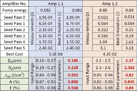
It is clear that a finer resolution – defined in this case as the step-size for scanning each interval – generates more accurate results by pinpointing precise input parameters while significantly increasing the execution time by the power of the number of scanning parameters (five in our case). To substantially increase this resolution while leveraging the execution time, we split the task into two stages. Initially, we run first a coarse search (e.g., with a resolution of 0.008) across the whole intervals of the rough known parameters of the amplifier. When the minimum coarse cost is found, a second run is performed with a much finer resolution (e.g., 0.002) over a tight interval (e.g.,
3.2.2 Modeling amplification chain
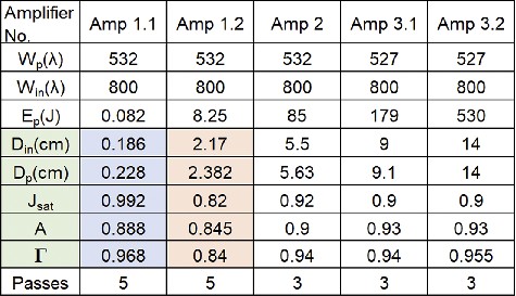
Table 2. Obtained input parameters, which describe each amplifier in the HPLS.
Table 2. Obtained input parameters, which describe each amplifier in the HPLS.
The technical description of our script is as follows: we utilize the
![]()
Figure 1.Logic scheme of the framework that models the amplification chain. The AMP function gathers data from the input matrix and calls PASS to perform the calculation.
To enhance the framework’s accuracy, we must account for a phenomenon present in Amp 1.2, thermal lensing. Pumping at high repetition rates and energy levels leads to the formation of a strong thermal lens. In the physical system, this thermal lens effect is compensated by injecting the seed with a relatively large divergence of
![]()
Figure 2.Simplified cross-sectional view of Amp 1.2’s geometrical model, illustrating beam clipping and divergence evolution during amplification. The red area shows the main beam propagation, green represents the pump diameter and the yellow arrow indicates the propagation direction. Calculated attenuation values for each pass are 0.71, 0.47, 0.71, 0.95 and 1.24. Note that the reduced diameter in the final pass enhances the extraction efficiency.
where
Given the characteristics of the beam in Amp 1.2, we approximate the evolution of the beam with a geometrical approach and neglect diffraction. By dividing the pump area by the seed area at the entrance of the crystal, we obtain our attenuation factor for each pass. This approach ensures that the simulated energy attenuation due to clipping closely matches the real behavior observed in Amp 1.2.
The last step is to deal with a particular feature present in the last three stages of amplification. Due to their large volume, these crystals are prone to transversal lasing, a parasitic process that involves the amplification of light traveling perpendicular to the crystal axis, leading to the fast depletion of gain[44]. To mitigate transversal lasing, several strategies were tested, among which the most effective is sequential pumping: the crystal is partially pumped a couple of nanoseconds prior to seed’s arrival and then pumped again after each pass, while the seed performs its roundtrip through the bow-tie. This drastically reduces the peak gain responsible for emergence of transversal lasing by extending it over the whole duration of the amplification process. This feature is particularly important to implement in our framework, as it substantially alters the extraction process and the residual gain. The particular pump energies prior to each pass are well-known, highly tunable parameters and are specific to each crystal. To implement this in the script, we simply populate a
3.2.3 Spectral domain analysis
The presented features accurately model the HPLS in the energy domain and serve as a solid basis for the integration of spectral analysis. To perform a spectral evolution across the amplification chain, we feed the script with a real spectrum of the seed extracted after the DAZZLER. The spectrum is then divided into 500 slices (or narrow wavelength ranges) and fed sequentially from ‘red’ to ‘blue’ into Equation (2) as
By integrating this feature into the amplification model and carefully tuning the input parameters, our framework achieves a faithful representation of the real laser system, capturing the nuances of the gain dynamics in both the energetic and spectral domains.
3.2.4 Calculating the B-integral
When all amplifiers have been accurately tuned and the amplification of the laser beam across the HPLS has been simulated, we can precisely track the intensity of the laser beam to calculate the accumulated B-integral. This is achieved by implementing Equation (1) within the amplification chain script.
The laser beam’s passage through the crystals is divided into 20 narrow spatial intervals for each pass. This resolution was carefully selected to balance computational efficiency with accuracy, as it faithfully captures the gradual increase in intensity during propagation through the crystals while keeping computation times manageable. Furthermore, tests with higher resolutions, such as 40 space intervals per crystal, revealed little difference in the calculated B-integral, confirming the adequacy of the chosen resolution.
The script iterates through all intervals and multiple passes for each crystal, accounting for their specific thicknesses. In addition to calculating the contribution to the B-integral from the crystals, the calculation also incorporates contributions from free propagation in air between passes and crystals, as well as from the 65 mm fused silica window used to inject the beam into the optical compressor placed in vacuum. Together, these components complete the total B-integral calculation. All the distances between passes and crystals were physically measured and entered into a table, which the script dynamically references during the computations.
3.2.5 Simulation of back-scattering amplification
After achieving a well-fitted model, the framework was extended to simulate BR propagation and amplification produced in an experiment by the interaction of the laser pulse with a thin foil target. This was done by seeding the beam back through the five amplifiers with an input energy level around hundreds of mJ, a value often observed from solid targets during the 10 PW experimental campaign utilizing our custom diagnostic devices built to capture BR. This BR amplification model takes into account the parameters stored in the input file (e.g., Table 2) while ignoring any pump energies. Only residual gain present in each crystal is considered. When estimating the residual gain, we must account for gain decay, which takes place during the beam’s round-trip travel from the crystal to the target and back. The distance from the target to the crystal ranges from 80 m for Amp 3.2 to 185 m for Amp 1.1, which corresponds to 530–1234 ns of beam travel time. From the fluorescence lifetime of the Ti:sapphire crystal
This gives us a map of gain decay for all the crystals present in the system (as shown in Figure 3) and concludes the optimization of our model to track BR amplification. In an attempt to reduce this BR amplification cascade while exploiting the advantages of reduced pumping, we explored, in our simulation, various pumping regimes of the HPLS to observe its effect on a seeded BR beam of 0.35 J (equivalent to
![]()
Figure 3.Map of gain decay (in percent) at the moment when the BR reaches each amplifier.
![]()
Figure 4.Monitoring BR amplification across the HPLS for the presented scenarios. The order of amplifiers is in line with the propagation of BR light.
![]()
Figure 5.Gain in the post-pulse regime in different pumping scenarios with their respective pumping energies. Note the residual gain is smaller in Amp 3.1 and Amp 3.2 for the full pump scenario due to the high extraction efficiency, despite being strongly pumped before the last pass. The order of amplifiers is in line with propagation of BR light.
4 Results
Utilizing the presented tools we have successfully managed to overlap our amplification simulation of the HPLS (i.e., from the DAZZLER to Amp 3.2) with its real counterpart in both spectral and energy content, as seen in Figures 6(a) and 6(b), respectively.
![]()
Figure 6.Normalized energy and spectral output of each amplifier in the chain. (a) Simulated amplification in the spectral domain. (b) Acquired spectra from each amplifier during the 10 PW experimental campaign. (c) Measured and simulated energy for each amplifier.
To track the spectral evolution of the BR beam, we utilized the real spectrum of a BR light captured for a 1 PW shot through the leakage of a mirror and fed it through the amplification chain in the reverse direction. In Figure 4 we observe that Amps 3.1 and 3.2 have a high extraction efficiency due to a strong seed regardless of pumping energy therein. The main beam depletes the crystals almost completely in its last pass despite the presence of sequential pumping, which facilitates a high influx of energy prior to the last pass. Moreover, their large operating beam diameters, 95 and 150 mm, respectively, are unsuitable for small traces of BR and only above 1.3% of back-reflected energy from the target (i.e., a factor of seven larger than what is presented) is the impact on the amplification process noticeable. It is clear that the pumping energy is inversely proportional to the residual gain in each crystal. Similar to amplification, the B-integral accumulation in the main beam is a cascade: facilitating a good extraction efficiency in an amplifier (i.e., raising energy output) will lead to faster B-integral accumulation in all subsequent amplifiers, which, when seeded strongly will further improve energy output and B-integral accumulation. Therefore, fully pumping all amplifiers leads to the lowest BR amplification and highest
Although the BR spectrum is highly sensitive to the target type and experimental interaction conditions, the available data indicate that in this case the band is compatible with the HPLS as its modulation is insufficient for further filtering by the optical compressor or the high-reflectivity dielectric mirrors within the system. However, in certain situations, the BR spectrum may undergo changes due to Doppler shifts, stimulated Raman scattering (SRS) or self-phase modulation (SPM)[46], in which case the alteration in its shape becomes more significant.
By employing the CPA technique, the main beam propagates through the HPLS with a positive temporal chirp, which is later nullified by the optical compressor; the BR beam, prior to entering the amplification chain, will pass a second time through the optical compressor, which will imprint a negative chirp. To emulated the present negative chirp in this spectral analysis, the BR pulse was fed from ‘blue’ to ‘red’. As such, in Figure 7 we see that the evolution of the BR spectrum through the amplification chain is low, which is likely correlated with the relatively low energy gained, with a slight blue-shift.
![]()
Figure 7.Evolution of the BR spectrum across the simulated amplification chain traveling from Amp 3.2 to Amp 1.1 with a negative chirp.
5 Conclusion
This study presents a comprehensive simulation framework for modeling both the main and BR beam amplification in high-power laser systems using the Frantz–Nodvik equation. The framework incorporates a robust optimization process to fine-tune amplifier parameters and is customized for their specific characteristics ensuring close alignment with physical measurements. This encompasses spatial seed clipping caused by induced beam divergence (Figure 2), which helps mitigate thermal lensing, as well as sequential pumping, which distributes the deposited energy throughout the entire amplification process. BR amplification simulation highlights the impact of residual gain and gain decay. Its implementation in Python allows for a versatile and iterative approach where certain key areas are targeted for the purpose of monitoring the energy and fluence of the main and BR beams traveling through the HPLS. This allows us to identify the most susceptible optical components to laser-induced damage while leveraging the gain in different stages of amplification for the best beam on target while operating in the safest manner. The standard for the rated energy that each area in the HPLS can handle is based on a conservative fluence value of 2 J cm
[1] D. Strickland, G. Mourou. Opt. Commun., 55, 447(1985).
[2] S. A. Gales, K. Tanaka, D. Balabanski, F. Negoita, D. Stutman, O Tesileanu, C. Ur, D. Ursescu, I. Andrei, S. Ataman, M Cernaianu, L. D’Alessi, I. Dancus, B. Diaconescu, N. Djourelov, D. Filipescu, P. Ghenuche, D. G. Ghita, C. Matei, K. Seto, M. Zeng, N. Zamfir. Rep. Prog. Phys., 9, 094301(2018).
[3] K. A. Tanaka, K. M. Spohr, D. L. Balabanski, S. Balascuta, L. Capponi, M. O. Cernaianu, M. Cuciuc, A. Cucoanes, I. Dancus, A. Dhal, B. Diaconescu, D. Doria, P. Ghenuche, D. G. Ghita, S. Kisyov, V. Nastasa, J. F. Ong, F. Rotaru, D. Sangwan, P.-A. Söderström, D. Stutman, G. Suliman, O. Tesileanu, L. Tudor, N. Tsoneva, C. A. Ur, D. Ursescu, N. V. Zamfir. Matter Radiat. Extrem., 5, 024402(2020).
[4] M. Borghesi, A. Mackinnon, D. H. Campbell, D. G. Hicks, S. Kar, P. K. Patel, D. Price, L. Romagnani, A. Schiavi, O. Willi. Phys. Rev. Lett., 92, 055003(2004).
[5] J. Kim, K. H. Pae, I. Choi, C. Lee, H. Kim, H. Singhal, J. Sung, S. Lee, H. Lee, V. Nickles, T. Jeong, C. Kim, C. Nam. Phys. Plasmas, 23, 070701(2016).
[6] C. Qin, H. Zhang, S. Li, N. Wang, A. Li, L. Fan, X. Lu, J. Li, R. Xu, C. Wang, X. Liang, Y. Leng, B. Shen, L. Ji, R. Li. Commun. Phys., 5, 124(2022).
[7] F. Brun, L. Ribotte, G. Boutoux, X. Davoine, P. E. Masson-Laborde, Y. Sentoku, N. Iwata, N. Blanchot, D. Batani, I. Lantuéjoul, L. Lecherbourg, B. Rosse, C. Rousseaux, B. Vauzour, D. Raffestin, E. D’Humières, X. Ribeyre. Matter Radiat. Extrem., 9, 057203(2024).
[8] T. M. Ostermayr, C. Kreuzer, F. S. Englbrecht, J. Gebhard, J. Hartmann, A. Huebl, D. Haffa, P. Hilz, K. Parodi, J. Wenz, M. E. Donovan, G. Dyer, E. Gaul, J. Gordon, M. Martinez, E. Mccary, M. Spinks, G. Tiwari, B. M. Hegelich, J. Schreiber. Nat. Commun., 11, 6174(2020).
[9] M. Mirzaie, C. I. Hojbota, D. Y. Kim, V. B. Pathak, T. G. Pak, C. M. Kim, H. W. Lee, J. W. Yoon, S. K. Lee, Y. J. Rhee, M. Vranic, Ó. Amaro, K. Y. Kim, J. H. Sung, C. H. Nam. Nat. Photonics, 18, 1212(2024).
[10] C. N. Danson, C. Haefner, J. Bromage, T. Butcher, J.-C. F. Chanteloup, E. A. Chowdhury, A. Galvanauskas, L. A. Gizzi, J. Hein, D. I. Hillier, N. W. Hopps, Y. Kato, E. A. Khazanov, R. Kodama, G. Korn, R. Li, Y. Li, J. Limpert, J. Ma, C. H. Nam, D. Neely, D. Papadopoulos, R. R. Penman, L. Qian, J. J. Rocca, A. A. Shaykin, C. W. Siders, C. Spindloe, S. Szatmári, R. M. G. M. Trines, J. Zhu, P. Zhu, J. D. Zuegel. High Power Laser Sci. Eng., 7, e54(2019).
[11] B. Shi, J. Li, S. Ye, H. Nie, K. Yang, J. He, T. Li, B. Zhang. Opt. Express, 30, 11026(2022).
[12] R. Dabu. Crystals, 9, 347(2019).
[13] V. Meghdadi, J.-P. Cances, F. Chevallier, B. Rojat, J.-M. Dumas. Ann. Télécommun., 53, 4(1998).
[14] T. Chapman, P. Michel, J.-M. G. Di Nicola, R. L. Berger, P. K. Whitman, J. D. Moody, K. R. Manes, M. L. Spaeth, M. A. Belyaev, C. A. Thomas, B. J. MacGowan. J. Appl. Phys., 125, 033101(2019).
[15] S. K. Mishra, A. Andreev, M. P. Kalashinikov. Opt. Express, 25, 11637(2017).
[16] O. Chalus, C. Derycke, M. Charbonneau, S. Pasternak, S. Ricaud, P. Fischer, V. Scutelnic, E. Gaul, G. Korn, S. Norbaev, S. Popa, L. Vasescu, A. Toma, G. Cojocaru, I. Dancus. High Power Laser Sci. Eng., 12, e90(2024).
[17] D. Kiefer. Relativistic Electron Mirrors(2015).
[18] A. Kon, M. Nishiuchi, Y. Fukuda, K. Kondo, K. Ogura, A. Sagisaka, Y. Miyasaka, N. P. Dover, M. Kando, A. S. Pirozhkov, I. Daito, L. Chang, I. W. Choi, C. H. Nam, T. Ziegler, H.-P. Schlenvoigt, K. Zeil, U. Schramm, H. Kiriyama. High Power Laser Sci. Eng., 10, e25(2022).
[19] D. Doria, M. O. Cernaianu, P. Ghenuche, D. Stutman, K. A. Tanaka, C. Ticos, C. A. Ur. J. Inst., 15, C09053(2020).
[20] I. Dancus, G. V. Cojocaru, R. Schmelz, D. Matei, L. Vasescu, D. Nistor, A.-M. Talposi, V. Iancu, G. P. Bleotu, A. Naziru, A. Lazar, A. Dumitru, A. Toma, M. Neagoe, S. Popa, S. Norbaev, C. Alexe, A. Calin, C. Ene, A. Toader, N. Stan, M. Caragea, S. Moldoveanu, O. Chalus, C. Derycke, C. Radier, S. Ricaud, V. Leroux, C. Richard, F. Lureau, A. Baleanu, R. Banici, A. Ailincutei, I. Moroianu, A. Gradinariu, C. Caldararu, C. Capiteanu, D. Ursescu, D. Doria, O. Tesileanu, T. Jitsuno, R. Dabu, K. A Tanaka, S. Gales, C. A. Ur. EPJ Web Conf., 266, 13008(2022).
[21] F. Lureau, G. Matras, O. Chalus, C. Derycke, T. Morbieu, C. Radier, O. Casagrande, S. Laux, S. Ricaud, G. Rey, A. Pellegrina, C. Richard, L. Boudjemaa, C. Simon-Boisson, A. Baleanu, R. Banici, A. Gradinariu, C. Caldararu, B. De Boisdeffre, P. Ghenuche, A. Naziru, G. Kolliopoulos, L. Neagu, R. Dabu, I. Dancus, D. Ursescu. High Power Laser Sci. Eng., 8, e43(2020).
[22] C. Radier, O. Chalus, M. Charbonneau, S. Thambirajah, G. Deschamps, S. David, J. Barbe, E. Etter, G. Matras, S. Ricaud, V. Leroux, C. Richard, F. Lureau, A. Baleanu, R. Banici, A. Gradinariu, C. Caldararu, C. Capiteanu, A. Naziru, B. Diaconescu, V. Iancu, R. Dabu, D. Ursescu, I. Dancus, C. A. Ur, K. A. Tanaka, N. V. Zamfir. High Power Laser Sci. Eng., 10, e21(2022).
[24] A. M. Val’shin, C. M. Pershin, G. M. Mikheev. Bull. Lebedev Phys. Inst., 46, 191(2019).
[25] E. G. Nagham, A. Sari, P. Venet, S. Genies, P. Azaïs. J. Energy Storage, 33, 102039(2021).
[26] D. Karimi, H. Behi, J. Van Mierlo, M. Berecibar. J. Energy Storage, 27, 3119(2022).
[28] S. Bock, F. M. Herrmann, T. Püschel, U. Helbig, R. Gebhardt, J. J. Lötfering, R. Pausch, K. Zeil, T. Ziegler, A. Irman, T. Oksenhendler, A. Kon, M. Nishuishi, H. Kiriyama, K. Kondo, T. Toncian, U. Schramm. Crystals, 10, 847(2020).
[30] K. K. Sharma. Optics: Principles and Applications(2006).
[31] V. Bagnoud, D. Zimmer, B. Ecker, T. Kuehl. Conference on Lasers and Electro-Optics, 1(2009).
[32] D. N. Schimpf, E. Seise, J. Limpert, A. Tünnermann. Opt. Express, 16, 10664(2008).
[33] N. V. Didenko, A. V. Konyashchenko, A. P. Lutsenko, S. Yu. Tenyakov. Opt. Express, 16, 3178(2008).
[34] F. Quéré, H. Vincenti. High Power Laser Sci. Eng., 9, e6(2021).
[35] A. A. Andreev, V. M. Komarov, A. V. Charukhchev, K. Yu. Platonov. Opt. Spectrosc., 102, 944(2007).
[36] C. Le Blanc, P. Curley, F. Salin. Opt. Commun. Eng., 131, 191(1996).
[37] D. F. Hotz. Appl. Opt., 4, 527(1965).
[38] F. Riehle. Frequency Standards: Basics and Applications(2003).
[40] L. M. Frantz, V. S. Nodvik. J. Appl. Phys., 34, 2346(1963).
[41] F. L. Pedrotti, L. M. Pedrotti, L. S. Pedrotti. Introduction to Optics(2017).
[43] S. Backus, C. G. Durfee, M. M. Murnane, H. C. Kapteyn. Rev. Sci. Instrum., 69, 1207(1998).
[44] F. Plé. , “Study of the transverse lasing in big size crystals of Ti:Sa. Application to the design of the peta-watt high-energy amplifier of the pilot laser of the LASERIX facility”, (Université Paris-Sud, 2007)..
[46] A. Giulietti, D. Giulietti. J. Plasma Phys., 81, 495810608(2015).
Tools
Get Citation
Copy Citation Text
Dmitrii Nistor, Alice Diana Dumitru, Christophe Derycke, Olivier Chalus, Daniel Ursescu, Catalin Ticos. Assessing optical damage risks by simulating the amplification of back-reflection in a multi-petawatt laser system[J]. High Power Laser Science and Engineering, 2025, 13(4): 04000e65
Paper Information
Category: Research Articles
Received: Apr. 9, 2025
Accepted: Jun. 24, 2025
Published Online: Sep. 24, 2025
The Author Email:

© Copyright 2018-2021 | Chinese Laser Press.
All Rights Reserved 沪ICP备15018463号-20