


Abstract
Imaging large cleared tissues requires scaling the throughput of imaging techniques. Light sheet microscopy is a promising technique for high-throughput imaging; however, its reliance on conventional microscope objectives limits the optimization of the trade-off between spatial resolution and field of view. Here we introduce curved light sheet microscope to perform optical sectioning with curved light sheets. This concept addresses the long-standing field curvature problem and lowers the barriers in designing high-throughput objectives. Leveraging a customized objective, the curved light sheet microscope achieves diffraction-limited resolution of 1.0 μm laterally and 2.5 μm axially, with uniform contrast over a field of view of more than 1 × 1 cm2. Our technique is also compatible with various tissue clearing techniques. We demonstrate that imaging an entire intact cleared mouse brain at a voxel size of 0.625 × 0.625 × 1.25 μm3 can be completed in less than 3 h, without the need for image tiling. We share a full optical description of the objective and report imaging of neuronal and vascular networks, as well as tracing of brain-wide long-distance axonal projections in intact mouse brains.
Main
The combination of light sheet microscopy and tissue clearing offers a powerful solution for examining the morphology and anatomy of large biological specimens1,2,3,4, and has unlocked a wide range of imaging applications in life sciences5,6,7,8,9,10,11,12,13,14,15,16,17,18,19. In recent years, continuous progress has been made in tissue clearing techniques20,21,22, enabling the clearing of ever-larger specimens ranging from intact mouse brains to entire mice and even entire human brains23,24,25,26,27. However, existing light sheet microscopes encounter a huge challenge when it comes to imaging these centimetre-sized specimens, primarily due to their reliance on conventional life science objectives. After all, most of these objectives are specifically designed for microscale imaging and tend to have a restricted space-bandwidth product (SBP, that is, the number of optically resolvable spots within the field of view), which necessitates a trade-off between spatial resolution and field of view28,29. For example, the multi-immersion ASI/Special Optics objective (54-12-8) for cleared tissue imaging offers submicrometre resolution, but its field of view is limited to 1 mm in diameter. Although image tiling is often used to overcome this barrier, it inevitably reduces imaging speed, generates more data and complicates subsequent image processing.
Scaling the throughput of light sheet microscopy requires scaling the SBP of imaging objectives. Considerable progress has recently been made in customizing objectives for high-resolution mesoscopic imaging14,30,31,32,33,34,35,36. A notable example is expansion-assisted selective plane illumination microscopy (ExA-SPIM), which has broken the volumetric imaging barrier by using a modified high-SBP industrial objective, enabling high-speed, -resolution and -contrast imaging of centimetre-scale cleared tissues14. However, in the design of mesoscopic objectives, field curvature—a centuries-old optical aberration—has emerged as a critical concern. This problem stems from the challenges of placing the mesoscopic field of view into a micrometre-scale depth of field. Field curvature does not aberrate the image but rather curves the image plane. Furthermore, improving flatness of the field requires more lens elements, which complicates the design and manufacture of the objectives. As a result, field curvature is rarely fully corrected. Even with commercial plan objectives, only 85% of the field of view is guaranteed within the depth of field37. The undesirable field curvature is indeed found in the multiple objectives tested in Benchtop mesoSPIM8, the high-throughput industrial objective in ExA-SPIM14, the mesolens for confocal microscopy30, the Schmidt objective32 and mesoscopic objectives for two-photon microscopy33,34,35. In point-scanning confocal and two-photon microscopes, the dish-shaped object plane has minimal impact as long as other aberrations such as coma and astigmatism are corrected; however, in light sheet microscopes with widefield camera detection, field curvature reduces resolution and contrast as parts of the field of view fall out of focus (Supplementary Fig. 1).
Here we introduce curved light sheet microscopy to address this long-standing problem. Unlike existing light sheet microscopes, curved light sheet microscope leverages a curved light sheet for optical sectioning, naturally diminishing the field curvature in imaging optics. More importantly, a curved object plane simplifies the design of high-SBP objectives, akin to natural systems such as human and aquatic eyes with curved retinas. Together with a stage scanning and line scan camera detection scheme38, we develop a high-throughput curved light sheet microscope for centimetre-sized cleared tissue imaging. We demonstrate its capabilities by imaging intact mouse organs prepared with various clearing techniques at micrometre resolution and without image tiling.
Results
High-SBP objective design
To scale the throughput of light sheet microscopy for imaging centimetre-sized cleared tissues, we set our goal to design a mesoscopic objective to meet four main requirements: (1) a numerical aperture of 0.25 with 8× magnification, enabling 1 μm diffraction-limited resolution suitable for mesoscale axonal mapping39; (2) a field of view exceeding 1 × 1 cm2 to enable imaging of entire mouse brains without the need for tiling; (3) a working distance of 2 cm to facilitate imaging of small intact organs such as mouse brains without requiring physical sectioning; and (4) compatibility with immersion media refractive indices from 1.33 to 1.60 to accommodate all tissue clearing techniques.
Taking advantage of the curved object plane, we designed a finite conjugate objective consisting of five lens elements to meet the four requirements (Fig. 1 and Supplementary Fig. 2a,b). The objective projects the magnified specimen’s image from the object to image plane without a tube lens. It is optimized to image specimens immersed in a medium-filled silica chamber, reducing the risk of objective contamination by immersion media. By tuning the working distance and refocusing, diffraction-limited performance can be achieved over a 13 mm diameter field of view for various immersion media and wavelengths from 460 to 700 nm (Supplementary Fig. 2c). The objective supports a SBP of more than 4 × 10⁸, with a mean SBP per lens element of 8.5 × 10⁷, which is about 10 times larger than conventional life science objectives (Supplementary Fig. 3). Beyond that, the simple design allowed assembling the objective in the laboratory to achieve diffraction-limited resolution across the centimetre-sized field of view (Fig. 1e,f, Supplementary Figs. 4 and 5, and Methods). The radius of the curved object plane varied with the refractive index of the immersion medium, and was measured to be 46.2 and 40.5 mm at n = 1.33 and 1.50, respectively, consistent with the simulations (Fig. 1d, Supplementary Fig. 2d and Methods). The resulted maximum focus shift was 135–155 μm, less than 2% of the 1 cm field of view.
Fig. 1: Overview of the curved light sheet microscopy.
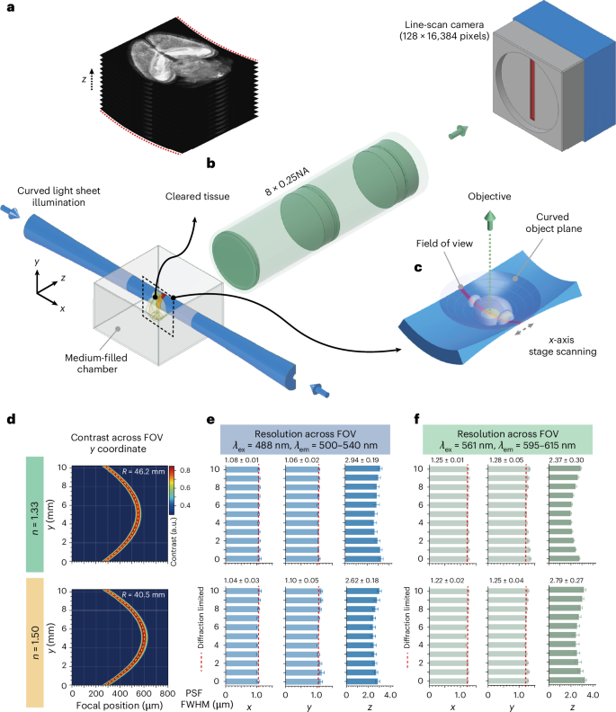
a, Schematic of the curved light sheet microscope in a standard double-sided illumination and horizontal detection architecture. The cleared specimen is mounted on a holder and immersed in the imaging buffer that fills a 50 × 50 × 50 mm3 sample chamber. Two-dimensional optical sections are captured by stage scanning the specimen along the propagation dimension of the laser (x axis). To image a z-stack, the specimen is moved along the optical axis of imaging optics (z axis). b, The z-stack captured is one-dimensionally curved along the y axis. NA, numerical aperture. c, Magnified view showcases the geometry of the curved light sheet, curved object plane, field of view and cleared specimen. d, Contrast at a spatial frequency of 100 line pairs per millimetre of the imaging optics measured for immersion media with refractive indices of 1.33 and 1.50; dashed yellow curves indicate the optimized curved light sheet illumination. e,f, Lateral and axial resolutions in terms of full-width at half-maximum (FWHM) of point spread functions (PSF) measured with 500 nm fluorescent beads under 488 nm (e) and 561 nm (f) laser excitations. The mean and s.d. of FWHMs were measured for 20–200 beads at each location; the FWHMs listed: mean ± s.d. (n = 11 locations). Throughout the 1 cm field of view (FOV), the average axial resolution is between 2.5 μm and 3.0 μm, and the lateral resolution is diffraction limited (1.0 μm and 1.2 μm for 500–540 nm and 595–615 nm fluorescence channels) for the example immersion media and laser excitations. λex, excitation wavelength; λem, emission wavelength.
Curved light sheet microscope design
We built the curved light sheet microscope with a standard horizontal illumination-detection architecture and a common sample mounting strategy5,6,7,8 (Fig. 1a–c, Supplementary Fig. 6 and Methods). Adapting a ring-focus generation technique from the laser machining industry40, we designed a curved light sheet illumination module where the radius of the light sheet plane can be flexibly adjusted to overlap with the curved object plane of the imaging objective (Supplementary Fig. 7 and Supplementary Note 1). The thickness and intensity of the light sheet were both uniform over a field of view of more than 1 cm along the y axis (Fig. 1e,f and Supplementary Fig. 8). Under 488 nm and 561 nm laser excitations, the light sheet’s thickness was 2.5–3.0 μm in working media where n = 1.33 and 1.50 (Fig. 1e,f), corresponding to a confocal range of ~80 μm along the x axis (Supplementary Fig. 9). The thin belt-shaped field of view was conjugated with a time delay integration (TDI) camera in image space. The 8× magnification of the objective implied a sampling rate of 0.625 μm per pixel in the x–y plane in object space, leading to a lateral imaging resolution of 1.25 μm limited by sampling based on the Nyquist sampling theorem (Supplementary Fig. 5).
We leveraged a simple and effective continuous stage scanning and TDI camera detection technique for imaging38. While operating, the camera is synchronized with the stage scanning along the x axis where the light sheet propagates. This mechanism suppresses out-of-focus fluorescence and achieves uniform axial resolution and contrast along the x axis as in the axially swept light sheet microscope (ASLM), where the rolling shutter of a scientific complementary metal–oxide–semiconductor (sCMOS) camera is synchronized with the axially swept light sheet to achieve optical sectioning15,41. The maximum field of view along x axis is defined by the effective scan distance of the stage and varies with scanning speed (Supplementary Fig. 10). At the speed of 1 cm per second mostly used in this work, the effective scan distance was approximately 2 cm, indicating the field of view along x axis of a single image can exceed the objective’s optical capacity.
The line scan rate of the TDI camera is coordinated with the scanning speed (Supplementary Fig. 10). When the stage scans at 1 cm per second, the line scan rate is 16 kHz, resulting in an imaging rate of 262 million pixels per second. Imaging a 1 × 1 cm2 optical section at this speed takes 1 s. For three-dimensional imaging, a motorized stage was used to scan along the axis of imaging optics (z axis). To use the full axial resolving power of the microscope, this stage advanced 1.25 μm for each optical section imaged. The captured image stack represents a one-dimensionally (along the y axis), gently curved cube in the object space (Fig. 1b). If necessary, the image stack can be uncurved with minimal computational cost, given the known radius of the curved object plane (Supplementary Fig. 11).
Imaging intact mouse organs cleared by various protocols
Using the curved light sheet microscope, we first imaged rigid specimens prepared by solvent-based (hydrophobic) clearing methods (Fig. 2a–e, Supplementary Video 1 and Supplementary Note 2). The polyethylene-glycol-associated solvent system (PEGASOS)-cleared26 Thy1-eGFP mouse brain was directly adhered to a sample holder and scanned for imaging in the immersion medium (Methods and Supplementary Fig. 6b,c). Due to brain shrinkage, the microscope's field of view along the y axis can cover the brain along the rostral–caudal axis. By scanning along the medial–lateral axis at 1 cm per second back and forth, it took about 3 h to image a whole brain with a voxel size of 0.625 × 0.625 × 1.25 μm3 in the object space, mainly depending on the thickness of specimen (Supplementary Table 1). Images of thin horizontal sections (9.69 × 10.24 mm2) were deconvolution-free and had a uniform contrast across the entire field of view (Fig. 2a and Supplementary Fig. 8). The near-isotropic resolution (where the axial resolution is two-times the lateral resolution) and stitching-free operation of the microscope revealed the brain-wide continuous axonal projections in all dimensions (Fig. 2a,b), with comparable image contrast from surface to deep layers of the brain (Fig. 2c,d). Both the lateral and axial resolution were well preserved at large depths, and axonal structures can be resolved (Fig. 2e). We also examined the vascular network of intact mouse brains cleared by PEGASOS (Fig. 2f–h, Supplementary Fig. 12, and Supplementary Videos 2 and 3). The microscope enabled detailed examination of the tree-like vascular branching systems (Fig. 2g), facilitating the visualization of continuous vascular branching structures and endothelial cells in three dimensions (Fig. 2h). We also imaged propidium-iodide-stained mouse brain and kidney cleared by immunolabeling-enabled three-dimensional imaging of solvent-cleared organs (iDISCO)42, revealing the distinct cell organizations across intact organs (Supplementary Figs. 13 and 14, and Supplementary Videos 4 and 5). Imaging an entire mouse brain typically produces ~1 TB of data. Note that conventional light sheet microscopes with a 10% tile overlap ratio for image tiling would generate at least 20% more data (Supplementary Note 3).
Fig. 2: Hydrophobic cleared tissue imaging by the curved light sheet microscope.
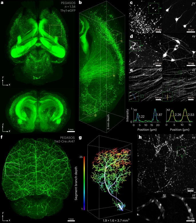
a, Lateral and axial maximum intensity projections (MIPs) of an entire intact PEGASOS-cleared Thy1-eGFP mouse brain. b, Rendering of a 1.6 × 1.6 × 5.0 mm3 subvolume indicated by the dashed yellow box in a. c,d, Representative lateral MIPs of subvolumes in the brain’s surface (c) and deep (d) layers; boxed areas are enlarged to the right to show individual neurons. e, Lateral and axial MIPs of a selected subvolume show fine structures of axonal fibre bundles. The line profiles across individual axons demonstrate the microscope’s resolving power at a large depth within the cleared brain; the FWHM values of Gaussian fits are displayed. f, Lateral MIP of an entire intact PEGASOS-cleared Tie2-Cre::Ai47 mouse brain. g, Close-up of the reconstructed vascular branching of a 1.9 × 1.6 × 3.7 mm3 subvolume indicated by the dashed white box in f. The vessels were reconstructed using an automatic filament tracing method in Imaris, and colour-coded on the basis of the segment branch depth, which represents the number of segment branch points in the shortest path from the starting point to a specific point within the branching structure. h, The lateral MIP of the subvolume indicated by the dashed white box in g; bottom panels show the magnified xy and yz views of the boxed area.
Next, we imaged soft specimens prepared by aqueous-based (hydrophilic) clearing methods (Fig. 3a–e and Supplementary Video 6). Mouse brain stained with propidium iodide and cleared by a commercial hydrophilic kit was embedded in a customized cuvette to prevent brain deformation during scanning (Methods and Supplementary Fig. 6b,c). Despite brain expansion post-clearing, the microscope can image the entire horizontal section in a single shot (15.31 × 10.24 mm2) by scanning along the rostral–caudal axis (Fig. 3a). The heterogeneous cell distribution across brain regions (for example, striatum, cerebral cortex, hippocampus and cerebellum) was clearly visible (Fig. 3b–e), enabling precise regional identification and structural analysis. We also imaged a CUBIC-cleared24 intact mouse kidney with feature regions identified from their delicate anatomic structures (Fig. 3f,g and Supplementary Video 7). Arteries were distinguished from veins by their thicker and more pronounced walls (Fig. 3h). Beyond that, distinct microstructures such as medullary rays, renal tubules and glomeruli were discernible in various anatomical regions (Fig. 3i–k). The high-contrast visualization of intact kidney would improve the systematic studies of kidney physiology and disease mechanisms.
Fig. 3: Hydrophilic cleared tissue imaging by the curved light sheet microscope.
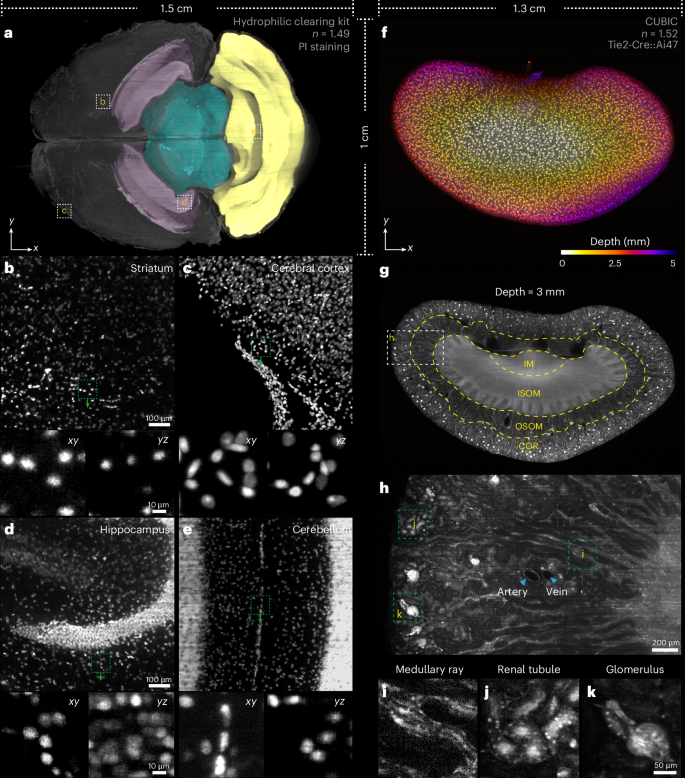
a, Lateral MIP of a 4.5-mm-thick horizontal section from the surface of an intact propidium iodide (PI)-stained mouse brain cleared by a commercial hydrophilic tissue clearing kit. The colour of each region represents anatomical annotations of representative brain regions obtained from the Allen Brain Atlas, including the hippocampus (pink), midbrain (blue) and cerebellum (yellow). b–e, Lateral MIPs of selected subvolumes in a to visualize the cell distributions in striatum (b), cerebral cortex (c), hippocampus (d) and cerebellum (e); the bottom panels show the magnified xy and yz views of the areas indicated by the dashed boxes. f, Lateral MIP of an entire intact CUBIC-cleared mouse kidney colour-coded by depth. g, A typical frontal section at 3 mm depth from the surface of the kidney. Dashed yellow lines delineate different subzones of the kidney. COR, cortex; OSOM, outer stripe of the outer medulla; ISOM, inner stripe of the outer medulla; IM, inner medulla. h, Enlarged views of the area indicated by the dashed box in g. i–k, Enlarged views of three typical anatomical structures: medullary ray (i), renal tubule (j) and glomerulus (k), as indicated by the dashed green boxes in h.
Axonal tracing with the curved light sheet microscope
Mapping axonal projections is challenging due to their thin diameter (<100 nm) and long distances (centimetres) across multiple brain areas. Light-microscope-based tracing techniques often use sparse labelling to minimize the close contacts between axons from different neurons43. This strategy relaxes the need for high spatial resolution to resolve overlapping axons and allows reconstruction of the morphology of individual neurons in their entirety with a voxel resolution of 1 μm (refs. 12,39). To demonstrate this capability, we imaged sparsely labelled neurons in the motor cortex of intact PEGASOS-cleared mouse brains, followed by reconstruction of neuron morphology using a semi-automated tracing method (Fig. 4, Supplementary Video 8 and Methods). The axonal projection patterns closely resembled those obtained with advanced imaging techniques involving extensive physical sectioning and image tiling, which can take several days to image an entire mouse brain44,45,46. The majority of neurons (12/15) projected from the injection site to the contralateral brain regions and exhibited mirror-symmetric axonal branching across the midline, whereas the remaining neurons projected to regions such as the medulla and thalamus (Fig. 4a). Examination of the axonal bundles near the midline highlighted the microscope’s ability to visualize axonal varicosities (Fig. 4b), whose distribution on the axonal main stem and collaterals can be crucial for understanding cortical connectivity47. The microscope preserved the image continuity and integrity of brain-wide axonal remote projections (Fig. 4c) and facilitated the inspection of whole dendrite trees, tracing of intertwined axonal branches, and identification of axonal terminals (Fig. 4d–f). Moreover, the curved light sheet microscope, compatible with multicolour imaging (Supplementary Fig. 15 and Supplementary Video 9), would allow the reconstruction of more neurons from a single brain without increasing reconstruction uncertainties. These capabilities underscored its potential to elucidate the brain’s wiring diagram.
Fig. 4: Tracing individual neurons with the curved light sheet microscope.
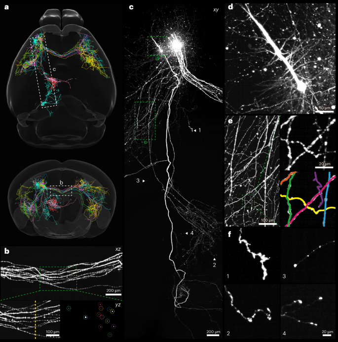
An intact mouse brain with sparse labelling of neurons in the motor cortex cleared by the PEGASOS method was imaged and traced. a, Horizontal and coronal overlay of 15 reconstructed neurons registered to an Allen Mouse Brain Atlas. b, The MIP showcases axonal bundles of 12 neurons projected from the injection site to the contralateral brain regions. The areas indicated by dashed boxes are enlarged to show dispersed axonal varicosities along the axons and cross-section view (dashed yellow line) of the axons. c, The MIP showcases the morphology of long-range projection neurons. d, The MIP of a dendritic tree. e, The MIP of tangled axon arbours. Boxed areas are enlarged to show the effectiveness of tracing; each identified segment is depicted in a different colour. f, Maximum intensity projections of four representative axon endings identified in the triangle indicated locations in c.
Discussion
In summary, we developed a high-throughput curved light sheet microscope for imaging centimetre-sized cleared specimens from various tissue clearing protocols. Optical sectioning with a curved light sheet could address the long-standing field curvature problem and lower the barrier to designing high-SBP objectives (Supplementary Note 4). Imaging an entire intact mouse brain using the curved light sheet microscope took a few hours with near-isotropic spatial resolution (1.25 μm laterally and 2.5 μm axially), and without tiling. The consistent image contrast across the field of view allowed us to visualize the fine neuronal and vascular structures, and trace multiple long-distance axonal projections over the mouse brains.
Although the current curved light sheet microscope leverages the simple customized objective, it is compatible with any objective as long as field curvature exists. For example, the Schmidt objective for two-photon imaging inherently has a spherical focal plane32. When paired with curved light sheet illumination, it could achieve higher throughput with widefield detection. Moreover, the curved light sheet illumination concept also applies to other light sheet imaging geometries. Switching the TDI camera from line scan to area mode would allow for the continuous recording of thin optical sections during stage scanning, as is done in the open-top and V-shaped light sheet microscopes9,10,11,12. This transition would expand the field of view from millimetre to centimetre scales, crucial for mapping large primate brains that require physical sectioning. Resolution of the curved light sheet microscope is approaching that of state-of-the-art tissue imaging techniques based on histological sectioning and block?face imaging39,48. However, the high-throughput light sheet microscope is sensitive to clearing quality. Insufficient clearing and minor remaining refractive index variations in the sample can result in fuzzy and blurry images4, as observed in the deep imaging of a propidium-iodide-stained mouse brain (Supplementary Video 6). Nevertheless, we anticipate that this limitation could be mitigated as tissue clearing techniques become more sophisticated to provide homogenous cleared specimens14.
Field curvature can also be addressed using curved image sensors or scientific camera arrays aligned to the curved image plane. In principle, these techniques could be coupled with planar light sheet illumination. Curved sensors, however, are still in the early stages of development and have fewer pixels and lower sensitivity than advanced planar image sensors49, and imaging with a scientific camera array would lead to a costly platform with a large footprint31,50. Furthermore, imaging large tissues prepared with different clearing protocols would benefit from techniques that can adapt to changes in field curvature, as demonstrated in this study. This demand poses a considerable challenge for curved sensors or camera arrays, necessitating further advancements.
The curved light sheet microscope uses a continuous stage scanning and TDI camera detection scheme to achieve optical sectioning by moving the specimen through a stationary light sheet38. This operation enables single-frame imaging with a field of view along the scan axis that exceeds the microscope’s optical capabilities, allowing for fewer image tiles when examining larger specimens (Supplementary Note 3). Beyond that, it simplifies the illumination optics compared with ASLM, which requires axial scanning mechanisms to generate axially swept light sheets15,41. Simple strategies such as using electrotuneable lenses are prone to spherical aberration8, necessitating more intricate remote focusing techniques for aberration-free operation13,15,41. Imaging speed of the current curved light sheet microscope is constrained by the imaging chamber’s dimensions and translational stage’s performance (Supplementary Fig. 10). As a result, the maximum attainable line scan rate is 48 kHz (Supplementary Fig. 16), notably lower than 300 kHz supported by the TDI camera. Nevertheless, this line scan rate translates to an imaging rate of 786 million pixels per second—surpassing the capabilities of light sheet microscopes using advanced sCMOS cameras and comparable with the ExA-SPIM platform employing a large-area CMOS camera14. Future hardware developments will increase the capacity of the current curved light sheet microscope. Besides sourcing faster stages and designing larger imaging chambers to increase the imaging rate, the potential developments include: (1) a TDI camera with more pixels along the y axis, which would allow the image resolution to reach the diffraction-limit, and imaging expanded tissues could further increase the resolution to resolve fine structures; (2) multi-channel fluorescence imaging would benefit from adding one or more lenses to the objective design to correct chromatic aberrations; and (3) replacing translational with rotational stage scanning could further boost throughput (Supplementary Fig. 17). Such improvements could open new avenues for large-scale imaging applications in neuroscience, development biology and three-dimensional pathology.
Methods
Curved light sheet microscope
A schematic of the curved light sheet microscope is shown in Supplementary Fig. 6a. The microscope was equipped with a single-mode fibre-coupled 200 mW, 488 nm laser (LBX-488-200-CSB-PPA, Oxxius) and a free-space output 150 mW, 561 nm laser (LCX-561L-150-CSB-PPA, Oxxius). The 488 nm laser was collimated by an achromatic doublet (AC254-150-A-ML, Thorlabs), whereas the 561 nm laser was expanded by a 20× beam expander (GBE20-A, Thorlabs). A flip mirror allowed for selection between the two lasers to image different fluorophores. The collimated laser beam (20 mm in diameter) was transformed into curved light sheet illumination through a y-focus cylindrical lens (LJ1558RM-A, Thorlabs), axicon (AX255-A, Thorlabs) and x-focus cylindrical lens (ACY254-050-A, Thorlabs) (Supplementary Fig. 7). A knife-edge prism mirror (MRAK25-P01, Thorlabs) was placed closely behind the axicon to split the ring-focus beam into two symmetrical halves for bilateral illumination. All cylindrical lenses were mounted in rotational mounts (CRM1PT/M, Thorlabs) to control their orientations precisely. To tune the curvature of curved light sheet illumination, the distance between the axicon and x-focus cylindrical lens was adjusted by moving the kinematic mirror pairs (M4-M5 and M2-M3) fixed on translation stages (XR25P/M, Thorlabs); the resulting distance change was compensated by moving the y-focus cylindrical lens fixed on an optical rail slider. The x-focus cylindrical lenses were mounted on two-axis translation stages (DT12XY/M, Thorlabs). Tilt angles of M3 and M5 were controlled by piezo inertia actuators (PIAK10, Thorlabs). This control was important for matching the curved light sheet illumination with the object plane of image optics and overlapping two light sheets from opposite side.
The belt-shaped field of view from the curved light sheet illumination was imaged by the customized high-SBP objective, which was mounted on a translation stage (XR25P/M, Thorlabs) and positioned horizontally on the optical table. Fluorescence was collected through an approximately 20-mm-thick immersion medium and a 2-mm-thick wall of the 50 × 50 × 50 mm3 fused silica chamber. The sample chamber was fixed on a translation stage (LX10/M, Thorlabs) to optimize the working distance for different immersion media. A 50 mm diameter bandpass filter (67-044 or 86-367, Edmund Optics) was placed behind the objective to reject excitation lasers, and fluorescence images were recorded with a TDI camera (HL-HM-16K30H-00-R, Teledyne DALSA). The camera featured a 128 × 16,384 array of 5 μm pixels and a maximum line scan rate of 300 kHz. At 8× magnification, the camera imaged a field of view of 80 μm × 10.24 mm with a sampling rate of 0.625 μm per pixel in the x–y plane in object space. The camera can operate in both the line scan and area readout modes. In the line scan mode, the 128-stage integration dramatically increased the effective exposure time when imaging moving specimens, which requires a constant velocity matching the camera’s line scan rate to prevent motion artifacts. In the area readout mode, it worked as a video camera for quick focus and optical alignment.
Specimens were mounted—using one of two methods, on the basis of their stiffness—to implement the stage scanning and TDI camera detection scheme (Supplementary Fig. 6b,c). Hard-cleared specimens from hydrophobic clearing methods were directly attached to a three-dimensional printed holder made of polylactic acid and placed in the immersion medium. BB-BED medium was used to adhere the specimens to the holder. The medium was composed of 47% (v/v) benzyl benzoate (BB), 48% (v/v) bisphenol-A ethoxylate diacrylate Mn 468 (BED) and 5% (v/v) quadrol supplemented with 2% (w/v) Irgacure 2959 as the ultraviolet initiator51. Soft-cleared specimens from hydrophilic clearing methods were embedded in the refractive index-matched hydrogels in a customized cuvette made of trimmed coverslips (~130 μm thick). The hydrogels were prepared by dissolving agarose into the tissue clearing solution. The sample holder was assembled on a Z-stage (MT1-Z8, Thorlabs) for z-axis scanning and an X-stage (LNR50M/M, Thorlabs) paired with a stepper motor actuator (DRV225, Thorlabs) for x-axis scanning.
The timing diagram for stage scanning and camera readout is shown in Supplementary Fig. 18. When the X-stage reached the targeted velocity and position, a TTL signal was sent to the TDI camera to initiate frame grabbing. The line scan rate of the camera and the number of lines per image on the x axis were predefined based on the scanning speed and field of view. Images were captured for both forward and reverse scans. Throughout the process, the Z-stage moved forward at a constant speed and advanced 1.25 μm for each image.
Data acquisition
Images were collected on a Windows-10-based workstation (Precision 7920 Tower, Dell) equipped with a motherboard (060K5C, Dell), processor (Intel Xeon Platinum 8260 CPU at 2.4 GHz, 48 CPUs) and 512 GB of RAM. One PCIe motherboard slot was used for the CameraLink frame grabber (Xtium2-CLHS PX8, Teledyne DALSA) to stream the raw images from the camera to RAM. The datasets were then saved to a 7 TB local disk in TIFF format. The speed of this transfer process outpaced the data generation speed of the microscope.
Objective screening
The high-SBP objective was designed with a simple lens architecture and assembled in the laboratory to reduce costs. It comprised one off-the-shelf singlet (LA1401-A, Thorlabs) and two customized doublets (Supplementary Fig. 19). We constructed a simple light sheet microscope to test the objective temporarily assembled on a customized V-mount to mitigate uncertainties from lens manufacturing processes. This setup enabled us to quickly evaluate various lens combinations from a selection of lens elements (Supplementary Fig. 4). The 488 nm laser was collimated with an achromatic doublet (AC254-150-A-ML, Thorlabs) and focused into a ~20-mm-wide light sheet with a cylindrical lens (LJ1695RM-A, Thorlabs). The tested objective was imaged from orthogonal direction, similar to a standard light sheet microscope. Subdiffraction-sized fluorescent beads were first imaged in the central field of view with the sample chamber filled with water (refer to the next section). We could promptly eliminate lens combinations with obvious optical aberrations by assessing the shape of imaged spots. The lateral PSF of the remaining lens combinations was calibrated to identify potential candidates. For lens combinations achieved diffraction-limited resolution, the lateral PSF was further calibrated over the field of view. The lens combination achieved uniform performance across the entire field of view was assembled in a customized objective barrel for the curved light sheet microscope.
Resolution quantification
Through imaging 500 nm fluorescent beads (F8813 and F8812, ThermoFisher) embedded in media with various refractive indices, we calibrated the performance of the microscope under 488 nm and 561 nm laser excitations. At n = 1.33, fluorescent beads at a concentration of 2% (v/v) were diluted 1:250, embedded in 0.4% agarose, and transferred into a square quartz capillary (0.5 × 0.5 mm2 cross-section) for imaging. At n = 1.50, the diluted fluorescent beads were evenly dispersed in a solution prepared by adding agarose to solution C (NH-CR-210701-L, Nuohai Life Science, Shanghai). The mixture was transferred into the square capillary and stored in a refrigerator at 4 °C for about 30 min before imaging. At n = 1.54, the fluorescent beads were diluted 1:250 in iohexol solution (HY-B0594, MedChemExpress) with the refractive index adjusted to 1.54. The mixture was transferred into the square capillary and stored in a refrigerator at 4 °C for about 2 h before imaging.
The capillary tube with fluorescent beads was clamped into a sample holder and positioned vertically in the chamber filled with immersion media. Aberrations from the 100-μm-thick capillary wall were minimal due to the small numerical aperture of the imaging optics9. A z-stack of 15 images of the beads with a step size of 0.5 μm was acquired with the TDI camera in area readout mode to measure the axial resolution (Fig. 1e,f). To assess the lateral optical resolution (Fig. 1e,f), images of the beads were captured over the entire field of view using an area scan camera (1.85 μm pixel size, acA4024-29 um, Basler) mounted on a vertical translation stage. The confocal range of the curved light sheet illumination along x axis was ascertained by imaging a z-stack of 15 images of the beads at a step size of 0.5 μm using the area scan camera (Supplementary Fig. 9). The contrast over the field of view was evaluated by imaging the beads with the TDI camera working in the line scan mode (Supplementary Fig. 8c). The image resolution for tissue imaging was measured by recording a z-stack of 100 images of the fluorescent beads at a step size of 0.5 μm with the TDI camera working in the line scan mode (Supplementary Fig. 5). The data were analysed using custom-written Python scripts. Point spread functions were fitted with Gaussian functions in x–y–z, and resolution was determined as FWHM of the fitted curves.
Field curvature quantification
We used a high-precision Ronchi ruling with 100 line pairs per mm (38-562, Edmund Optics) to measure the field curvature of the objective8. The ruling was mounted on the Z-stage, immersed in the imaging buffer, aligned with the imaging path, and transilluminated with uniform LED lighting. Using the TDI camera, we captured 1,000 images at 1 μm intervals while the ruling moved through the curved object plane. The image stack was divided into 80 subregions along the y axis, and the contrast in each subregion was calculated for all images according to the following formula:
where Imin and Imax were determined by the 1st and 99th percentiles of intensity within the image, respectively. This process generated the two-dimensional contrast map and the contrast across focus in each subregion was fitted with a Gaussian function to find its focal position with maximum contrast. A circle function was used to fit the 80 focal positions pinpointed to extract the radius of the curved object plane. Curved light sheet illumination with this radius would allow all-in-focus imaging across the field of view.
Animals
All experimental procedures and protocols related to the use of mice were approved by the Institutional Animal Care and Use Committee of the Chinese Institute for Brain Research, Beijing (CIBR), in accordance with the governmental regulations of China.
Sample preparation
Stereotaxic AAV injection
For sparse labelling, stereotaxic AAV injection52 was performed on C57BL/6J mice aged 6–8 weeks old. A mixture of AAV2/9-hsyn-Cre (titre = 13 × 1012, diluted 10,000×) and AAV2/9-EF1α-DIO-mScarlet (titre = 8.7 × 10¹²) at a 1:1 ratio was injected into the secondary motor cortex (anteroposterior = 2.34 mm from bregma; mediolateral = −1.0 mm; dorsoventral = −1.5 mm). For two-colour labelling, stereotaxic AAV injection was performed on C57BL/6J mice aged ten weeks old. A combination of pAAV-hSyn-Cre (titre = 13 × 1012), pAAV-DIO-CAG-eGFP (titre = 17 × 1012, diluted 1,000×) and pAAV-DIO-CAG-mito-mScarlet AAV2/9 (titre = 17 × 1012, diluted 1,000×) was injected into the primary motor cortex (anteroposterior = 0.61 mm from bregma; mediolateral = 1.25 mm; dorsoventral = −1.3 mm). After injection, the micropipette remained in place for 10 min before withdrawal. Mice were allowed to recover for three weeks before being killed.
PEGASOS mouse brain clearing
The brains of a Thy1-eGFP-M mouse (P90), a Tie2-Cre::Ai47 mouse (P50), a Pitx2-Cre::Ai47 mouse (P35) and the AAV-injected mice were cleared with PEGASOS26. The brains were dissected and fixed in 4% PFA at 4 °C overnight and decolorized with a 25% (w/v in H2O) quadrol solution (122262, Sigma-Aldrich) at 37 °C for 2 days. They were then immersed in gradient delipidation solutions at 37 °C for 1 day per concentration: 30%, 50% and 70% tert-butanol (tB, 360538, Sigma-Aldrich) (v/v in H2O), each supplemented with 3% (w/v) quadrol to adjust the pH. The brains were then dehydrated in a medium containing 70% (v/v) tB and 30% (w/v) quadrol at 37 °C for 2 days. Finally, the brains were immersed in BB-PEG clearing medium (n = 1.543) at 37 °C until fully transparent—typically within 1 day. The BB-PEG clearing medium was composed of 75% (v/v) benzyl benzoate (W2131802, Sigma-Aldrich) and 25% (v/v) PEGMMA500 (447943, Sigma-Aldrich), supplemented with 3% (w/v) quadrol. Cleared samples were preserved in BB-PEG solution at 4 °C, which was also used as the imaging medium.
IDISCO mouse kidney and brain clearing
The kidney of a C57BL/6J mouse (P60) and the brain of a Thy1-eGFP mouse (P5) were cleared with a modified iDISCO protocol53. The organs were dissected and then fixed in 4% PFA overnight at 4 °C. Samples were washed three times with 1× PBS at room temperature and dehydrated via serial incubations (20%, 40%, 60%, 80%, 100% and 100% methanol in double-distilled H2O, 1 h each). Delipidation was performed overnight in 66% dichloromethane (DCM) in methanol at room temperature. After two washes with 100% methanol (2 h each), samples were pre-cooled at 4 °C and then bleached in 5% hydrogen peroxide in methanol overnight at 4 °C. Rehydration was performed via serial incubations in 80%, 60%, 40% and 20% methanol in double-distilled H2O, followed by one incubation in PBS and two incubations in PTx.2 (0.2% TritonX-100 in 1× PBS) at room temperature (1 h each). Samples were stained with propidium iodide (1:50, 40710ES03, Yeasen Biotechnology, Shanghai) in PTx.5 (0.5% TritonX-100 in 1× PBS) supplemented with 0.05% sodium azide for 3 days at 42 °C, with shaking at 60 r.p.m., followed by two washes with PTx.5 (1 h each), and an overnight incubation at room temperature. Samples were further washed four times with 1× PBS and dehydrated via serial incubations (20%, 40%, 60%, 80%, 100% and 100% methanol in double-distilled H2O, 1 h each). Delipidation was repeated in 66% DCM in methanol for 3 h at room temperature, followed by two washes in 100% DCM (15 min each). Finally, samples were cleared by Dibenzyl ether (108014, Sigma-Aldrich) at room temperature.
Hydrophilic kit mouse brain clearing
The brain of an eight-week-old mouse was cleared with a commercial kit (NH-CR-210701-L, Nuohai Life Science, Shanghai). The brain was dissected and fixed in 4% PFA at 4 °C overnight and washed twice with 1× PBS for 2 h each at room temperature. Delipidation was performed by immersing the brain in a 9:1 mass ratio mixture of solutions A and B for 6 days at 37 °C, with daily solution replacement. After delipidation, the brain was washed three times in 1× PBS for 2 h each at 4 °C. Immunostaining was performed by incubating the brain in propidium iodide solution (1:50, 40710ES03, Yeasen Biotechnology, Shanghai) for 2 days at 37 °C with shaking at 60 r.p.m., followed by three washes in 1× PBS for 2 h each at room temperature. Refractive index matching was achieved by treating the brain with solution C at 25 °C for 2 days with shaking. For hydrogel embedding, 2% agarose was dissolved in solution C and added to the customized cuvette, which then partially solidified at 4 °C for 30 min; the brain was then gently placed into the cuvette, submerged in the gel and cooled at 4 °C for 2 h before imaging.
CUBIC mouse kidney clearing
The kidney of a Tie2-Cre::Ai47 mouse (P60) was cleared with CUBIC24. The kidney was dissected and fixed in 4% PFA at 4 °C overnight. The sample was washed three times in 1× PBS for 2 h each and pre-delipidated with 50% CUBIC-L medium (T3740, TCI Chemicals) in double-distilled H2O overnight at 37 °C. Delipidation was performed in CUBIC-L for 4 days at 37 °C, with the solution refreshed on days 1 and 2. After three washes in 1× PBS for 2 h each, refractive index matching was performed using 50% CUBIC-R+ medium (T3741, TCI Chemicals) for 1 day at room temperature. The sample was further incubated in CUBIC-R+ medium until fully transparent. For hydrogel embedding, 2% agarose was dissolved in CUBIC-R+ medium and added to the customized cuvette. The sample was immersed in the mixture and cooled until it was fully embedded in the gel. The gel-embedded sample was then stored at room temperature until imaging.
Single-neuron morphological reconstruction
The neuronal reconstruction was semi-automatedly performed with the Lychnis software12 (https://github.com/SMART-pipeline/Lychnis-tracing). Each neuron was initially reconstructed by a human annotator, which was followed by dual-round proofreading and revising processes by two other independent annotators. Neurons with broken neurites were excluded from the analysis. All of the 15 neurons analysed in this study were validated by consensus among the three independent human annotators. The autofluorescence background of the brain from the dataset (10 × 10 pixels binning) was rendered and registered to an Allen Mouse Brain Common Coordinate Framework v.3 (CCFv3, 10 μm resolution) with publicly available software54 (https://github.com/brainglobe/brainreg). The resulting transformations were used to map the reconstructed neurons to the Allen Mouse Brain Atlas.
Data processing
Images were visualized and processed using Imaris (Oxford Instruments) and Fiji55. Unless stated otherwise, all images presented here were unprocessed raw images without smoothing, denoising and deconvolution.