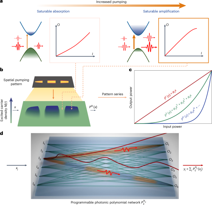
a, Pump-dependent photonic nonlinearity in an active semiconductor such as InGaAsP. When InGaAsP is unpumped or weakly pumped, a substantial portion of electrons resides in the valence band. Their transition to the conduction band, excited by the signal light, results in intrinsic absorption. Due to finite carrier populations, the transmission of the signal light is intensity-dependent, reflecting saturable absorption. As the pump power increases, more carriers become excited in the conduction band. Their recombination with holes in the valence band provides optical gain to the signal light, leading to saturable amplification. b, Spatial distribution of excited carriers controlled by the external pumping pattern, incident perpendicular to the sample plane, as indicated by the orange solid arrow. The combination of spatially varying pumping levels across the 2D space yields strong nonlinear light–matter interactions, enabling the reconfiguration of transmission curves programmed into different polynomial functions for the signal propagating from left to right. c, Programmable polynomial functions, showing that both the degree N and the l-order coefficients α_l of the synthesized polynomial functions can be tuned by spatial pumping patterns. d, Field-programmable photonic polynomial microprocessor for on-chip information processing and in situ learning. Nonlinear connections between arbitrary input and output ports can be established to create a fully connected integrated photonic network with complete programmability (indicated by the green lines). Selective spatial pumping allows for individual tuning of polynomial connections. For example, two different photonic connections (I₃ to O₆ and I₃ to O₁) with different spatial pumping strategies are demonstrated: segmented pumping ( to ) alternates between amplification (marked in orange) and absorption (marked in blue), causing oscillations in signal power along the propagation direction (illustrated by the light trail above the connection), which favours high-order polynomials with enhanced nonlinearity. In contrast, continuous pumping ( to ) leads to a monotonic increase in light power along propagation (also indicated by the light trail above), yielding low-order polynomials close to a linear function.

To validate field-programmable photonic nonlinearity and its ability to reconfigure polynomial functions, we fabricated the sample (see Methods) on a 250-nm-thick thin film of InGaAsP (Fig. 2a). The signal light with a wavelength of approximately 1,550 nm is generated by a micro-ring laser on the input side, with its transmission monitored using a grating coupler on the output side for free space detection. The I/O connection, that is, the InGaAsP thin film in between, remains lithographically unpatterned, such that carrier excitations within InGaAsP are purely modulated by 2D distributed external optical pumping, at a wavelength of 1,064 nm, programmed by a spatial light modulator (see Methods). In this work we focus on the reconfiguration of enhanced saturable absorption which, compared with saturable amplification, offers convex transmission curves with higher-N polynomials commonly used in data-intensive applications. To facilitate a strong interaction between signal light and local carriers within the semiconductor, it is important to maintain the intensity of signal light near the transparency intensity along the entire pathway of an I/O connection. Note that the available local carrier density regulates the imaginary part of the susceptibility of the semiconductor, consequently influencing its associated optical gain/loss coefficient (see Supplementary Section 1). Therefore, the spatial modulation between intense and weak external pumping emerges as efficient in managing local light intensity and its nonlinear interaction with carriers, effectively reshaping the transmission curve. In this scenario, a periodic modulation of pump light in space between the input and the output is employed under the overall envelope of the elliptically shaped pumping profile derived from an adjoint method³⁴, which is conveniently programmed with two parameters: the duty cycle β, defined by the ratio of the pumped area in a spatial period (β = a/b in Fig. 2a), and the total pumping power  along this single I/O connection. With our focus on the convex functions, the nonlinearity in transmission curves is dominated by saturable absorption; therefore, the decrease in the value of β provides more unexcited carriers, leading to the reconfigurable synthesis of the nonlinear transmission functions continuously from nearly linear to strongly nonlinear (Fig. 2b). Simultaneously, by elevating  to counterbalance absorption stemming from the expanded unpumped region, the signal intensity can be maintained at a level for efficient carrier dynamics of saturable absorption throughout the I/O connection, allowing the strategy to be deployed for networks with varying scales.

Fig. 2: Reconfigurable polynomial I/O connection.

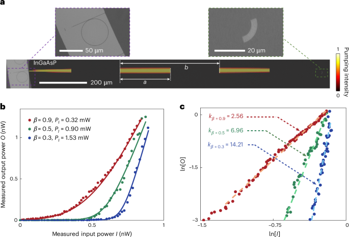
a, Optical microscope image of the fabricated sample used for characterizing the reconfigurable polynomial I/O connection, alongside the overlay of the spatial modulation of optical pumping applied in experiments. Here, a denotes the length of a pumping segment, whereas b represents the length of a spatial period. The two upper insets show the input unit comprising a micro-ring laser coupled to a straight waveguide connected to the unpatterned InGaAsP region and a grating coupler in InGaAsP designed for output detection. b, The relationship between output and input power under different pumping scenarios, highlighting the reconfigurable polynomial I/O connection controlled by the duty cycle β. The overall pumping power  is adjusted to maintain a consistent output signal intensity across different scenarios. The solid lines are the simulation results from the travelling-wave model, showing remarkable consistency with experimental measurements. c, The relationship between output and input power in a logarithmic scale, directly showing the dominant polynomial order of the synthesized polynomial function (estimated via slopes). The fitting is applied to  > 0.05 nW ( > −3) to avoid the influence of noise at low signal levels.

The minimum of β is set by the maximum gain provided by the material and in this work is positioned at 0.2. The dominant polynomial order of the corresponding transmission curve is mainly determined by the value of β, as can be seen clearly from the slope in the logarithmic scale (Fig. 2c). In principle, the obtained nonlinear function should take the form of a polynomial comprising multiple orders, but the dominant order can serve as an effective indicator for quantifying the nonlinearity of the function. Evidently, the predominant polynomial term can be effectively tuned from low to high orders with decreasing β, culminating in a polynomial order as high as N ≈ 14 with β = 0.3. Furthermore, it is crucial to highlight that concave-shaped nonlinear functions with N < 1—as well as more complex polynomials with precisely tailored combinations of different orders—can also be achieved (see Supplementary Section 2), with the ability to reconfigure their polynomial orders in real-time. By leveraging the convenient programmability in polynomial orders, we can extend our capabilities further to synthesize even more complex nonlinear functions through cascading the photonic polynomial connections, tackling increasingly intricate computing tasks. Also note that the result shown in Fig. 2b closely resembles the widely used rectified linear unit (ReLU)³⁵ function in deep neural networks, thereby being able to serve as fixed activation functions in conventional neural networks (see Supplementary Section 3). Its integration with linear networks holds considerable promise if heterogeneously integrated with a variety of platforms, particularly with silicon photonics through mature III–V/silicon integration³⁶.

Instead of conventional neural network models with elementwise nonlinear activation functions typically sandwiched between adjacent linear networks, our focus is to field-program optical polynomial functions in real-time, where polynomial functions are directly employed to connect neurons for deploying polynomial networks. Polynomial networks, which leverage the richer information provided by polynomial functions, can outperform purely linear matrix operations in various contexts, as demonstrated below. To deploy the field-programmable photonic polynomial network, we developed an iterative training algorithm (see Supplementary Section 4) to optimize the pumping pattern controlling the spatial modulation of carrier excitations within the 2D InGaAsP thin film. In our experiments, each I/O connection is individually controlled by the two parameters mentioned previously, that is, the duty cycle β_i,j and the pump power  (for the connection from input j to output i), and the iterative algorithm simultaneously updates both parameters for the optimization of all connections in the network.

To exemplify the superior performance of field-programmable photonic nonlinearity, we start with a benchmark two-class classification problem involving two input variables, where a synthetic dataset consists of two features in the input layer, labelled as  and  (Fig. 3a). The boundary between the two classes forms a curve within the feature vector space, showing an intrinsic nonlinear characteristic that can only be addressed using a nonlinear network. In experiments, we deployed a field-programmable 2 × 2 photonic network to execute a nonlinear transformation, directing the processed signal to the two output ports corresponding to the two classes (Fig. 3b). The feature vector (, ) was encoded with normalized emission power from two micro-ring lasers at inputs. The predicted class was directly indicated by the higher intensity observed between the two output channels. Initially, a symmetric pumping pattern was configured with a uniform duty cycle and total pumping power for all four nonlinear I/O connections. In each training epoch, following the measurements of all 300 data points, a loss function  was calculated, where O_tgt and O_mea are the target and measured output vectors defined as the power of each output port, respectively. The polynomial function of each connection () was then updated. After 40 epochs, the classification accuracy reached 97.3%. In the feature vector space of the outputs, the two classes were predominantly separated, demonstrating effective distinguishability (Fig. 3c). When transforming back to the input vector space, only a few misclassifications near the boundary were observed (Fig. 3d). It is important to note that, for the intrinsic nonlinearity of this benchmark classification problem, these two classes cannot be effectively distinguished by any linear network. For comparison, a control experiment with a linear network was also conducted, resulting in a final accuracy of approximately 64.5% (see Supplementary Section 5).

Fig. 3: In situ training with field-programmable photonic nonlinearity for benchmark problem solving.

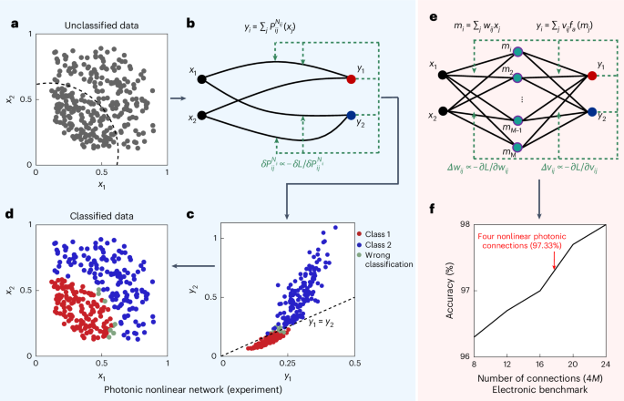
a, Feature vector space of input data where two distinct datasets reside in two domains demarcated by a curved boundary. b, Training schematic for the photonic polynomial network illustrating the process of in situ training using field-programmable photonic nonlinearity. Each nonlinear connection (solid black lines) takes individual programming in a parallel manner according to feedback loops (green dashed lines) derived from measurement results. c, Post-training classification results where the classification outcomes are delineated by a straight line of . d, Input vector space post-training, where the clear separation of two classes represents effective performance. e, Training schematic for a computer-trained digital neural network outlining the training process. Nonlinear activation functions are applied to  neurons in the intermediate layer. The network is trained by adjusting the weights ( and ) in the linear transformations within each layer, as depicted by the green dashed lines. f, Classification accuracy as a function of computer-trained network complexity. Remarkably, it reveals that 20 trainable linear connections are required to barely surpass the experimental performance of our single-layer photonic polynomial network with only four connections.

The same task was also tested using digital conventional neural networks with one intermediate layer, where fixed nonlinear ReLU functions (f_α) were applied to each neuron between two linear networks (Fig. 3e). Two fully connected matrices  and  are digitally trained using a computer, resulting in 4M trainable weights with M neurons in the middle layer. The final accuracy achieved by the digital networks largely depends on the total number of connections (Fig. 3f). Despite using a much simpler architecture with only four connections, the photonic polynomial network can achieve a classification accuracy that is comparable with that attained through digital computation, which uses a conventional neural network with 16 to 20 linear connections and applies nonlinear activation to four neurons. This highlights the intrinsic higher information density provided by the direct programming of polynomial functions.

To harness the dynamic reconfiguration capabilities of field-programmable photonic nonlinearity for accelerating computing tasks, we performed in situ training for the Iris dataset³⁷ (see Supplementary Section 6), which is one of the most recognized datasets in the field of machine learning. The dataset consists of 150 samples across three iris flower species: Iris setosa (I. setosa), Iris versicolor (I. versicolor) and Iris virginica (I. virginica), each characterized by four features: sepal length, sepal width, petal length and petal width, which form the input feature vector. Notably, I. versicolor and I. virginica are challenging to distinguish using a linear network due to their similar feature distributions. A fully connected 4 × 3 photonic polynomial network is conducted on our device (Fig. 4a), where four micro-ring lasers are excited to form the input vector, with the power of each micro-ring laser corresponding to the respective feature vector element (see Methods). In the output layer, the three classes are categorized as three output channels, representing I. setosa (), I. versicolor () and I. virginica (). The predicted class is determined by identifying the output channel with the highest intensity. At the core of the system is the unpatterned InGaAsP thin film that can host field-programmable photonic nonlinearity, where distributed carrier excitations enable direct programming of the polynomial network and real-time learning in a fully connected architecture. Two training strategies are employed to validate the importance of nonlinear connections: one using a nonlinear polynomial network trained on both duty cycle β and power  for each individual I/O connection, and the other employing a linear network with a fixed β = 1 for all connections (see Supplementary Section 7), while keeping all other parameters constant. Evidently, the nonlinear network exhibits a much lower training loss upon convergence, indicating a substantial performance enhancement (Fig. 4b). Upon the completion of the training, the nonlinear network has achieved a final classification accuracy of 96.7% for both the training and testing datasets (Fig. 4c,d), outperforming the linear network, which reaches only 85.8% accuracy for the training dataset and 86.7% for the testing dataset (Fig. 4e,f). The experimental results are consistent with the digital network simulations (see Supplementary Section 6). In addition to accuracy, another important performance indicator is confidence, which reflects how strongly the model believes that an input belongs to a given class. For the nonlinear network (Fig. 4g), the output power corresponding to the correct class is much higher than that of the other two classes, as shown by the power distribution across the output ports. By contrast, for the linear network (Fig. 4h), the output powers for I. versicolor (green) and I. virginica (blue) are comparable across output ports  and , indicating difficulty in clearly distinguishing between the two classes. To quantify the distinguishability, we define a parameter D for a sample belonging to class l as D = p_l − max{p_m,m ≠ l}, where  is the normalized power ratio of the output port l. For correctly classified samples, D represents the difference in normalized powers between the correct port and the most misleading incorrect port. The average distinguishability for I. versicolor and I. virginica is D_nl = 0.12 for the nonlinear network, in stark contrast to D_l = 0.02 for the linear network.

Fig. 4: Photonic polynomial networks for iris flower classification.

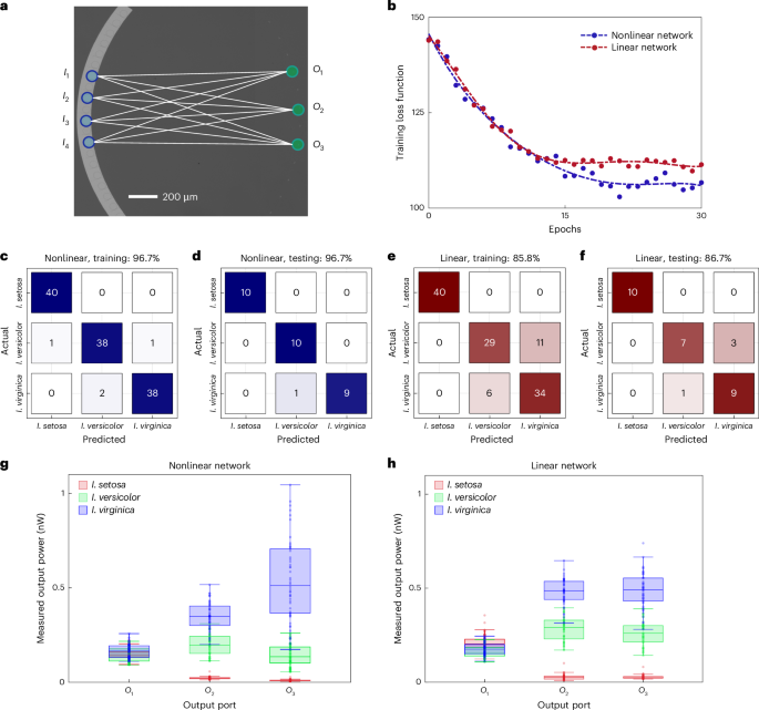
a, The schematic depicts a single layer of a 4 × 3 network designed for the iris flower classification task. The four-element feature vectors are encoded by the four micro-ring lasers on the left side (marked with blue circles). The output signal is measured through three grating couplers, each corresponding to a different iris class. b, Evolution of the loss function during the training of nonlinear (blue) and linear (red) networks. In the nonlinear network (blue), both the duty cycle β and power  are trainable across all 12 connections, whereas in the linear network (red), only the power of individual connections is trainable, with the duty cycle β fixed at . Both strategies start with the same initial pumping pattern; slight differences in the loss function at the beginning of training are attributed to fluctuations in the pumping pattern generation and camera detection during extensive dataset measurements. The dashed lines are polynomial fittings of the experimental data (denoted by dots). c–f, Confusion matrices of the training (c,e) and testing (d,f) datasets for the nonlinear (c,d) and linear (e,f) networks. The value in each box represents the number of samples. g,h, Box charts of the measured power at the output ports for all data after training for nonlinear (g) and linear (h) networks. For each class, the boxes indicate the interquartile range with the central line indicating the median. The coloured whiskers extend from the upper (lower) quartile to the non-outlier maximum (minimum), marked by the horizontal lines. Outliers are defined as data points more than 1.5 times the interquartile range from the edges of the boxes.

Achieving high distinguishability is essential for ensuring robust and scalable performance in analogue photonic computing systems. As the network size and complexity grow, this capability becomes even more critical, enabling photonic nonlinear polynomial networks to handle intricate computational tasks with greater reliability and precision. To demonstrate this, we performed in situ training for speech command recognition³⁸ using a 16 × 4 fully connected polynomial network. The data were pre-processed, and a subset was created to match the scale of the network (see Supplementary Section 8). A dataset of 480 audio samples was randomly divided into 360 samples for training and 120 samples for validation, representing four distinct words: ‘Bird’, ‘Happy’, ‘House’ and ‘Tree’. To reduce redundancy in the raw audio data, the intensity distribution across 16 frequency bands was extracted as the feature vector for each sample (q_s for data s). These feature vectors were then encoded as input signals and sequentially fed into the polynomial network. After training, the nonlinear network achieved a classification accuracy of 92.5% and 91.7% on the training and testing datasets, respectively (Fig. 5c,d), also outperforming the linear network (see Supplementary Section 9), which attained accuracies of 89.2% and 86.7% on the training and testing datasets, respectively (Fig. 5e,f). These results are consistent with our digital simulations (see Supplementary Section 8) and highlight the advantages of incorporating nonlinearity into the network. This result marks the first demonstration of intricate computations using a photonic polynomial network, made possible by the direct programming of photonic nonlinear I/O connections. By unlocking new levels of computational power and versatility in integrated photonics through reconfigurable nonlinear light–matter interactions, our approach paves the way for advancing more complex, real-world applications (see Supplementary Section 10).

Fig. 5: Photonic polynomial networks for speech command recognition.

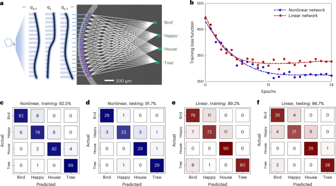
a, Speech command recognition task in a 16 × 4 photonic polynomial network. Fourier transform is applied to each audio data (s) to encode it as intensity distribution across 16 frequency bands (depicted by the blue bars) generated from 16 micro-ring lasers on the left side of the sample, forming the input feature vector. The output signal is measured through four grating couplers corresponding to ‘Bird’, ‘Happy’, ‘House’ and ‘Tree’, respectively. b, Evolution of the loss function during training nonlinear (blue) and linear (red) networks. Dashed lines represent polynomial fitting of the experimental data denoted by dots. c–f, Confusion matrices of the training (c,e) and testing (d,f) datasets for the nonlinear (c,d) and linear (e,f) networks.

We have demonstrated a groundbreaking advancement in field-programmable photonic nonlinearity through quantum control of carrier dynamics within an active semiconductor thin film, executing polynomial functions with a simpler architecture and faster processing speed than the electronic counterpart (see Supplementary Section 11). The precise manipulation of spatially excited carrier densities enables the realization of highly reconfigurable polynomial photonic connections. Distinguished from the replications of well-developed electronic architectures on photonic platforms, our work serves as a pioneer in the exploration of photonic paradigms specifically tailored for computing with light, accounting for the intrinsic disparities between photons and electrons. By facilitating direct, real-time programming of polynomial networks, our demonstrated field-programmable photonic nonlinearity represents a significant leap forwards in photonic computing and its integration with reconfigurable computing architectures.