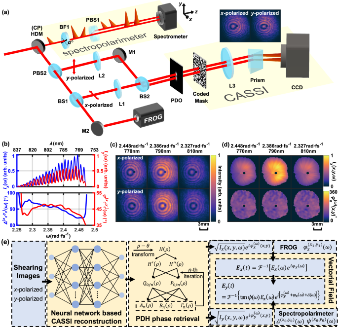
a The schematic experimental setup. The spectropolarimeter consists of a birefringent crystal (BF1), a polarization beam splitter (PBS1), and a homemade two-channel spectrometer. The coded aperture snapshot spectral imager (CASSI) includes a coded mask, an imaging lens L3, an angularly dispersive prism, and a charge-coupled device camera (CCD). CP: checking point; HDM: holed drilled mirror; PBS2: polarization beam splitter; BS1, BS2: beam splitters; M1, M2: reflective mirror; L1, L2: imaging lens; PDO: point-diffraction object; FROG: Frequency-resolved optical gating. b Spectropolarimeter results ??(?) and ??(?) (top panel) at (?0,?0), and reconstructed frequency-resolved polarization parameters ?(?0,?0)(?) and Δ(?0,?0)(?) (bottom panels). Corresponding wavelengths are labeled on top. c CASSI reconstructions for ?- (top row) and ?-polarized (bottom row) point-diffraction holograms at wavelengths of 770 nm (left column), 790 nm (middle column), and 810 nm (right column), with corresponding angular frequencies marked on top. d Point-diffraction holographic reconstruction results for ?-polarized light, including intensity ??(?,?,?) (top row) and spatial phase profiles φ?(?)(?,?) (bottom row) at wavelengths of 770 nm (left column), 790 nm (middle column), and 810 nm (right column). Data with normalized intensity <0.1 is neglected. e The 3D spatiotemporal vectorial optical field reconstruction procedure.

For the remaining light reflected from the hole-drilled mirror (HDM), ?- and ?-polarized light components are separated by a polarization beam splitter (PBS2), and transmitted through convex lenses L1 and L2, respectively. We place a point-diffraction object (PDO) close to the rear focal planes of L1 and L2, to measure spectrally resolved spatial phase profiles φ?(?)(?,?) and φ?(?)(?,?) of ?- and ?-polarized light. In actual experiments, the point-diffraction object is implemented by a liquid-crystal spatial light modulator, introducing two phase modulation spots (180 μm-diameter) at spatial centers of ?- and ?-polarized light, respectively. The wavelength dependency of the spatial light phase modulation is considered in spatial phase recovery, only introducing negligible contrast variations among point-diffraction holograms for different spectral components. As the modulated beams are imaged by L1 and L2 from the checking point (CP) to the coded mask (a chromium-coated fused silica plate with a random binary pattern), point-diffraction holograms with concentric ring patterns are formed. The 3D spatiospectral intensity profiles of ?- and ?-polarized point-diffraction holograms are captured by the CASSI system^23,24, i.e., spatially modulated by the coded mask, imaged by a lens L3, spectrally sheared by the prism, and finally captured or spectrally integrated by a charge-coupled device (CCD, Fig. 1a inset). Here, the combination of point-diffraction holography and CASSI for 3D phase retrieval of φ?,?(?)(?,?) in the spatiospectral domain is an interferometric compressive imaging approach, different from previous 3D scalar field measurements relying on the whole-beam diffraction^{17,18,19,29,30}. Therefore, any phase or polarization singularity in the 3D vectorial field profile of complicated structured light can be reliably resolved.

To process the compressive sensing data, we use a standard CASSI reconstruction algorithm based on self-supervised neural networks (details in the “Methods” section)³⁹ to reconstruct the ?- and ?-polarized 3D spatiospectral point-diffraction holograms (Fig. 1c). Spatiospectral intensity profiles ??(?,?,?) and ??(?,?,?), as well as spatial phase profiles φ?(?)(?,?) and φ?(?)(?,?) can in principle be retrieved from corresponding point-diffraction holograms in Fig. 1c using commercial fringe analysis software⁴⁰, but we developed a simple iterative algorithm instead (Fig. 1d, details in the “Methods” section). Finally, a small portion of the ?-polarized laser field transmits through the splitting mirror (BS1) and the reflective mirror (M2) to a home-made non-collinear frequency resolved optical gating (FROG) device⁴¹, and a genetic algorithm is applied to reconstruct the spectral phase φ?(?1,?1)(?) at an arbitrarily chosen spatial position (?1,?1)^30,42. Now 3D spatiospectral phase profile of ?-polarized laser field is φ?(?,?,?)=[φ?(?)(?,?)−φ?(?)(?1,?1)]+φ?(?1,?1)(?).

Now we can calculate the 3D spatiospectral and spatiotemporal light field profiles. Fourier transformation along the spectral domain on ??(?,?,?)eiφ?(?,?,?) yields the 3D spatiotemporal profile ??(?,?,?)eiφ?(?,?,?) of the ?-polarized light field. For the ?-polarized light, the 3D spatiospectral phase profile is φ?(?,?,?)=[φ?(?)(?,?)−φ?(?)(?0,?0)]+φ?(?0,?0,?)+Δ(?0,?0)(?), and the amplitude one is ??(?,?,?)=??(?,?,?)??(?0,?0,?)/??(?0,?0,?)×tan??(?0,?0)(?). The complex amplitudes of ?- and ?-polarized light components unambiguously determine the 3D spatiospectral polarization state with a method different from previous approaches using metasurfaces^36,37. The 3D spatiotemporal field profile ??(?,?,?)eiφ?(?,?,?) is obtained again through Fourier transformation on ??(?,?,?)eiφy(x,y,?), and complete light field information is obtained using Eq. (1). The data reconstruction procedure of the 3D spatiotemporal vectorial optical field is systematically illustrated in Fig. 1e, including all key calculation steps mentioned above.

To prove the concept, we first generate less structured light fields with 3D homogeneous linear, circular, and elliptical polarization states, and test the capability of resolving 3D spatiotemporal amplitude, phase, polarization, and wavelength information. An ?-polarized, 800 nm, 40 fs laser pulse coming from a 1 kHz Ti:Sapphire laser amplifier transmits through a half-wave plate (WPZ2325-795 from Union Optics Inc.) whose optical axis is −15° to the ?-direction, so the output laser field is expected to be linearly polarized along -30° to the ?-direction. Figure 2a shows the actual field profile along the linear polarization direction with the carrier laser frequency reduced by 0.4 times for clear illustration. Meanwhile, the polarization directions of the laser field at selected time slices are labeled by white arrows around −30° to the ?-direction in Fig. 2b. The 3D intensity profile has a 38 fs temporal duration.

Fig. 2: High-dimensional one-shot optical sensing of homogeneously polarized light.

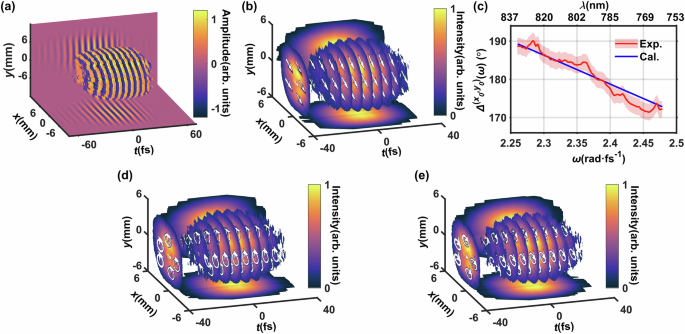
a The 3D spatiotemporal optical field profile of a femtosecond laser pulse with linear polarization −30° to the ?-direction. The carrier laser frequency is reduced by 0.4 times for clear illustration. b The 3D spatiotemporal polarization direction (white arrows) and intensity (color map) profiles of the linearly polarized femtosecond laser field for selected time slices. c The polarization parameter Δ(?0,?0)(?) describing the spectral phase difference between ?- and ?-polarized components of the linearly polarized femtosecond laser pulse, the red line is for the experimental (2.17° standard deviation shown in pink area) and the blue line for the calculation results. d and e The same as b, but for right-rotating circular (d) and left-rotating elliptical (e) polarizations.

Detailed studies show that the measured polarization phase difference Δ(?0,?0)(?) changes from 190° for the 2.26 rad/fs frequency component (834 nm wavelength) to 172° for the 2.48 rad/fs one (760 nm wavelength) (Fig. 2c red), consistent with calculations based on the half-wave plate refractive index provided by the supplier (Fig. 2c blue). Thus, the chromatic dispersion of the incident half-wave plate introduces wavelength–polarization coupling of a supposed linearly polarized light, illustrating the high-dimensional resolving power of the proposed scheme. In the time domain, the polarization state at each time slice is averaged over the entire spectral bandwidth, showing little variation.

We then use quarter-wave plates to generate light fields with right-rotating circular and left-rotating elliptical polarization, and Fig. 2d and e show their 3D spatiotemporal polarization states (white arrows) and intensities (color maps). For the elliptical polarization case, the white arrows form ellipses rotating along the left-hand direction, and their long axes are 20° to the ?-direction, consistent with the design. Moreover, the light chirality in each case is unambiguously determined, justifying the genuine 3D one-shot polarization resolving capability for arbitrary light, instead of simple specialized cases such as linear polarization^33,34,35.

High-dimensional one-shot sensing of 2D structured light fields

As reviewed in ref. ¹, 2D structured light refers to optical fields with a transversely ?–? spatial pattern of amplitude, phase, or polarization. One typical example is the optical vortex, which has a spiral spatial phase integer time of the azimuthal angle, physically representing the orbital angular momentum (OAM) of photons⁴³. As optical vortices have broad applications in optical communications^44,45,46, biological microscopy⁴⁷, and quantum computation⁴⁸, spatiotemporal vortices beyond 2D have even been demonstrated^49,50.

Here we conduct the high-dimensional one-shot sensing of a 2D optical vortex with +1 orbital angular momentum, which is generated by propagating an ?-polarized femtosecond laser pulse through a quarter-wave plate and a vortex retarder (Fig. 3a). Figure 3b shows the reconstructed 3D intensity profile, and as expected intensity singularities near the center of the beam profile are observed. The laser field has spatiotemporally homogeneous linear polarization along the ?-direction (Fig. 3b white arrows). The spatial phase profiles of the vortex field at different time slices (?= −25, −15, −5, 5, 15, 25 fs are presented in the polar coordinate (Fig. 3c). In each time slice, the phase linearly increases with the polar angle from 0° to 360°, indicating the +1 optical angular momentum as designed. In addition, the 360°–0° phase jump azimuthal angles at the radial position of 4.8 mm are plotted in Fig. 3(d) as a function of time, and the phase jump angle decreases rapidly from 170° to 140° during ?= −15 to 15 fs, but gradually during other time periods. The nonlinear decrease of the phase jump angle is related to the residual third-order spectral dispersion of the laser field. This complicated spatiotemporal phase–wavelength coupling effect proves the necessity of global high-dimensional optical field sensing.

Fig. 3: High-dimensional one-shot optical sensing of optical vortex fields.

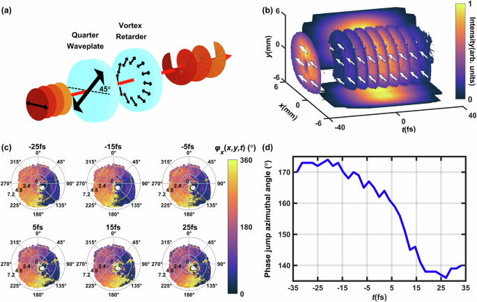
a The schematic experimental setup for optical vortex generation, including a quarter-wave plate and a vortex retarder. b The 3D spatiotemporal polarization direction (white arrows) and intensity (color map) profiles of the optical vortex field. c Spatial phase profiles of the optical vortex field at time slices of −25, −15, −5, 5, 15, 25 fs. Data corresponding to normalized intensity <0.2 is neglected. The small white regions in the centers are singularity points, and those on the lower right side are due to the hole-drilled mirror HDM. d The 360°−0° phase jump azimuthal angle as a function of time, the radial position is 4.8 mm.

Another two important types of 2D structured light are radially and azimuthally polarized beams, which are applied to represent a novel complete set of quantum states^51,52, accelerate high-energy particles⁵³, image through biological tissues⁵⁴, and fabricate three-dimensional microstructures^55,56. We first generated the radially polarized beam by replacing the quarter-wave plate in Fig. 3a with a half-wave plate, whose optical axis is along the ?-direction and parallel to the incident laser’s linear polarization direction.

Figure 4a shows the reconstructed 3D spatiotemporal polarization directions, which are radially distributed (white arrows), as well as the intensity profile whose temporal duration is 40 fs close to the linearly polarized incident laser field. Intensity singularities are observed again along the two transversely spatial dimensions, similar to the case of an optical vortex. We take a representative time slice of the light field at ?= 0 fs, and ?(?,?,?=0) defining the angle between the local polarization direction and the ?-direction, which is plotted in the polar coordinate of Fig. 4b, confirming the radial polarization distribution. The phase difference Δ(?,?,?=0) between ?- and ?-polarization components is also plotted in Fig. 4c, around 360° in the 1st and 3rd quadrants but 180° in the 2nd and 4th quadrants as expected. Small discrepancies of Δ(?,?,?=0) from the designed values represent small ellipticities of the light field.

Fig. 4: High-dimensional one-shot optical sensing of radially and azimuthally polarized beams.

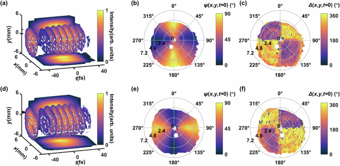
a The 3D spatiotemporal polarization direction (white arrows) and intensity (color map) profiles of the radially polarized beam. b The polarization parameter ?(?,?,?=0) describing the amplitude ratio angle between ?- and ?-polarized light components of the radially polarized beam. c The polarization parameter Δ(?,?,?=0) describing the phase difference between ?- and ?-polarized light components of the radially polarized beam. d–f The same as a–c, but for the azimuthally polarized beam.

To generate an azimuthally polarized beam, we rotate the half-wave plate with its optical axis along the ?-direction. The 3D spatiotemporal intensity and polarization profile are illustrated in Fig. 4d, showing polarization vectors pointing azimuthally. This observation is further corroborated by the detailed polarization angle map ?(?,?,?=0) and the phase difference map Δ(?,?,?=0) at the time slice of ?= 0 fs (Fig. 4e, f), consistent with the designed azimuthal polarization state.

High-dimensional one-shot sensing of structured light fields beyond 2D

Control of structured light beyond 2D involves the manipulation of optical fields along the longitudinal temporal dimension. One typical example of such longitudinally structured light is the so-called polarization-gating field, which has counter-rotating circular polarization states at the leading and trailing edges of the pulsed light field, but is linearly polarized in the narrow central temporal region⁵⁷. Polarization-gating fields have been applied for isolated attosecond electron and light pulse generation^58,59, and chiral detection of biological molecules⁶⁰. As shown in Fig. 5a, we generate the polarization-gating field by transmitting an ?-polarized 40 fs incident laser pulse through a birefringent crystal (~0.6 mm quartz with its optical axis at 45° to ?), introducing a 16 fs time delay between ordinary and extraordinary fields. Then a quarter-wave plate converts ordinary and extraordinary fields into left- and right-circularly polarized ones respectively, but in their temporally overlapping area, left- and right-circularly polarized fields coherently add up to form linear polarization.

Fig. 5: High-dimensional one-shot optical sensing of polarization-gating fields.

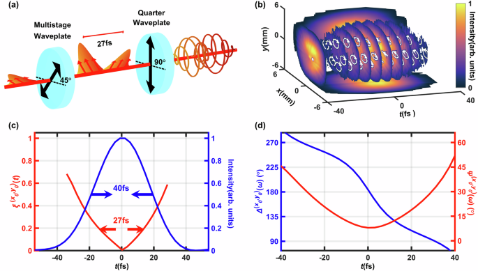
a Experimental setup for the polarization-gating field generation, including a birefringent quartz crystal (optical axis is 45° to the ?-direction) and a quarter-wave plate (optical axis is along ?-direction). b The 3D spatiotemporal polarization direction (white arrows) and intensity (color map) profiles of the polarized-gating fields. c The temporal intensity (blue line) and ellipticity ?(?0,?0)(?) (red line) of the polarization-gating field at the point (?0,?0). d The time-dependent polarization parameters ?(?0,?0)(?) and Δ(?0,?0)(?) at the point (?0,?0).

The high-dimensional one-shot sensing result of the polarization-gating field is illustrated in Fig. 5b, including the 3D intensity and polarization state distributions. Based on the spatiotemporal polarization state profile, the measured laser field polarization changes from left-rotating elliptical at ?= −30 fs to linear in a narrow time window around ?= 0 fs, and further to right-rotating elliptical as ? increases, until finally right-circular at ?= 40 fs. These experimental observations are consistent with the polarization-gating field theory⁵⁷. As high harmonic attosecond light pulse generation efficiency is directly related to the ellipticity of the driving laser field, we calculate the time-dependent ellipticity of the measured polarization states of the vectorial polarization-gating laser field using ?=sin−1(sin?2?sin?Δ) (Fig. 5c). A gated temporal region with ?<0.2 for efficient high harmonic generation has a temporal duration is 27 fs, consistent with the theoretical prediction of 27 fs⁶¹. Further extending our proof-of-concept measurement to polarization-gating fields based on broadband few-cycle laser pulses is also feasible, thanks to the broad spectral coverage of CASSI.

Moreover, in most isolated attosecond light pulse generation experiments where the polarization gating technique is applied, the accurate linear polarization direction in the temporally narrow central gated region, as well as the generated attosecond light polarization direction, are hardly determined, because they are extremely sensitive to the thickness of the birefringent quartz crystal, ambient temperature, and other unexpected factors. Therefore, such ignorance of the polarization state of the attosecond light pulse degrades not only the accuracy of its spectral characterization using a grating, but also the degree of coherence after beam transportations through grazing reflective extreme ultraviolet optics for downstream applications. In contrast, Fig. 5d explicitly shows the longitudinally time-dependent polarization parameters ?(?0,?0)(?) and Δ(?0,?0)(?), and the direction of the central linearly polarized gated field (?) is 8° to the ?-direction. As far as we know, it is the first time to experimentally determine the polarization gating direction, potentially benefiting attosecond sciences.